Fun with Filters and Frequencies
Building convolution from scratch, then using it to find edges, sharpen photographs, hide one image inside another, and blend images without a visible seam.
All three of my numpy convolutions match scipy.signal.convolve2d to within 1.3 × 10⁻¹⁵ on 126 test cases. Smoothing before differentiating cut isolated edge noise on the cameraman by 8.5×. For hybrid images, placing the two filter cutoffs about 4× apart in frequency was what made the illusion switch cleanly. For blending, blending each frequency band with its own blurred mask removed the seam in every blend.
Fun with Filters
Building intuition for 2D convolution, starting from the humble finite difference \(D_x = [1, 0, -1]\), \(D_y = D_x^\top\).
Part 1.1: Convolutions from Scratch!
A 2D convolution slides a flipped kernel over the image and takes a weighted sum at every position:
The minus signs are the flip. Without it the operation is cross-correlation, which gives the same answer only for symmetric kernels. For an antisymmetric kernel like \(D_x = [1, 0, -1]\), skipping the flip would negate every derivative.
Padding and output modes
All three versions share one helper. It zero-pads the image by \(k-1\) pixels on each side, which is exactly what full mode needs, and then records where the requested output starts inside that padded result. same starts \(\lfloor (k-1)/2 \rfloor\) pixels in, which is the centering scipy uses, so even-sized kernels line up too. valid starts \(k-1\) pixels in. Doing it this way means the padding logic is written once and the three loop structures below differ only in how they walk over the data.
def _prepare(image, kernel, mode):
    image = np.asarray(image, dtype=np.float64)
    kernel = np.asarray(kernel, dtype=np.float64)
    H, W = image.shape
    kh, kw = kernel.shape
    padded = np.zeros((H + 2 * (kh - 1), W + 2 * (kw - 1)))
    padded[kh - 1:kh - 1 + H, kw - 1:kw - 1 + W] = image

    if mode == 'full':
        start, shape = (0, 0), (H + kh - 1, W + kw - 1)
    elif mode == 'same':
        start, shape = ((kh - 1) // 2, (kw - 1) // 2), (H, W)
    elif mode == 'valid':
        start, shape = (kh - 1, kw - 1), (H - kh + 1, W - kw + 1)
    else:
        raise ValueError(f'unknown mode {mode!r}')
    flipped = kernel[::-1, ::-1]
    return padded, flipped, start, shape
Four loops, two loops, and a second kind of two loops
The four-loop version is the definition written out literally: one loop per output row and column, and one per kernel row and column. The standard two-loop version keeps the pixel loops and replaces the inner pair with a single vectorized multiply-and-sum over the patch. I also wrote the other way to cut the loop count: loop over the kernel taps instead, and at each tap add one shifted, scaled copy of the whole image. That is still two loops, but now each iteration is a full-image numpy operation instead of a tiny per-pixel one.
def conv2d_four_loops(image, kernel, mode='same'):
    padded, k, (r0, c0), (oh, ow) = _prepare(image, kernel, mode)
    kh, kw = k.shape
    out = np.zeros((oh, ow))
    for i in range(oh):
        for j in range(ow):
            acc = 0.0
            for u in range(kh):
                for v in range(kw):
                    acc += k[u, v] * padded[r0 + i + u, c0 + j + v]
            out[i, j] = acc
return outdef conv2d_two_loops(image, kernel, mode='same'):
padded, k, (r0, c0), (oh, ow) = _prepare(image, kernel, mode)
kh, kw = k.shape
out = np.zeros((oh, ow))
for i in range(oh):
for j in range(ow):
patch = padded[r0 + i:r0 + i + kh, c0 + j:c0 + j + kw]
out[i, j] = np.sum(patch * k)
return outdef conv2d_tap_loops(image, kernel, mode='same'):
padded, k, (r0, c0), (oh, ow) = _prepare(image, kernel, mode)
kh, kw = k.shape
out = np.zeros((oh, ow))
for u in range(kh):
for v in range(kw):
out += k[u, v] * padded[r0 + u:r0 + u + oh, c0 + v:c0 + v + ow]
return outCorrectness and runtime
Before timing anything I checked every version against scipy.signal.convolve2d with zero fill. The test used random images and kernels in all three modes, including even-sized and non-square kernels (1×3, 2×2, 4×3, 2×6, …). All 126 cases agree, and the worst difference is 1.3 × 10⁻¹⁵, which is floating-point rounding. Timings below are on my 376×480 grayscale selfie (180,480 pixels), same mode, best of several runs:
| Kernel | Four loops | Two loops (pixels) | Two loops (taps) | scipy | Max |ours − scipy| |
|---|---|---|---|---|---|
| 9×9 box | 4.61 s | 682.2 ms | 22.7 ms | 30.2 ms | 1.4 × 10⁻¹⁵ |
| Dx (1×3) | 221.9 ms | 655.1 ms | 1.2 ms | 2.2 ms | 0 |
| Dy (3×1) | 245.6 ms | 653.2 ms | 1.1 ms | 3.8 ms | 0 |
The four-loop version takes 4.61 s for the 9×9 box because Python pays interpreter overhead on every one of the roughly 15 million multiply-adds. Vectorizing the patch sum makes it 6.8× faster, but the pixel loop still makes one numpy call per output pixel. For the 3-tap \(D_x\) that call overhead costs more than the arithmetic it replaces, so the "faster" two-loop version is actually 3.0× slower than four loops. The tap loop avoids that overhead: 81 full-image operations for the box filter, 22.7 ms in total, 203× faster than four loops and even 1.3× faster than scipy's direct C implementation on this kernel. What matters is how much work each iteration of the loop you keep does, not just how many loops there are.
Boundary handling
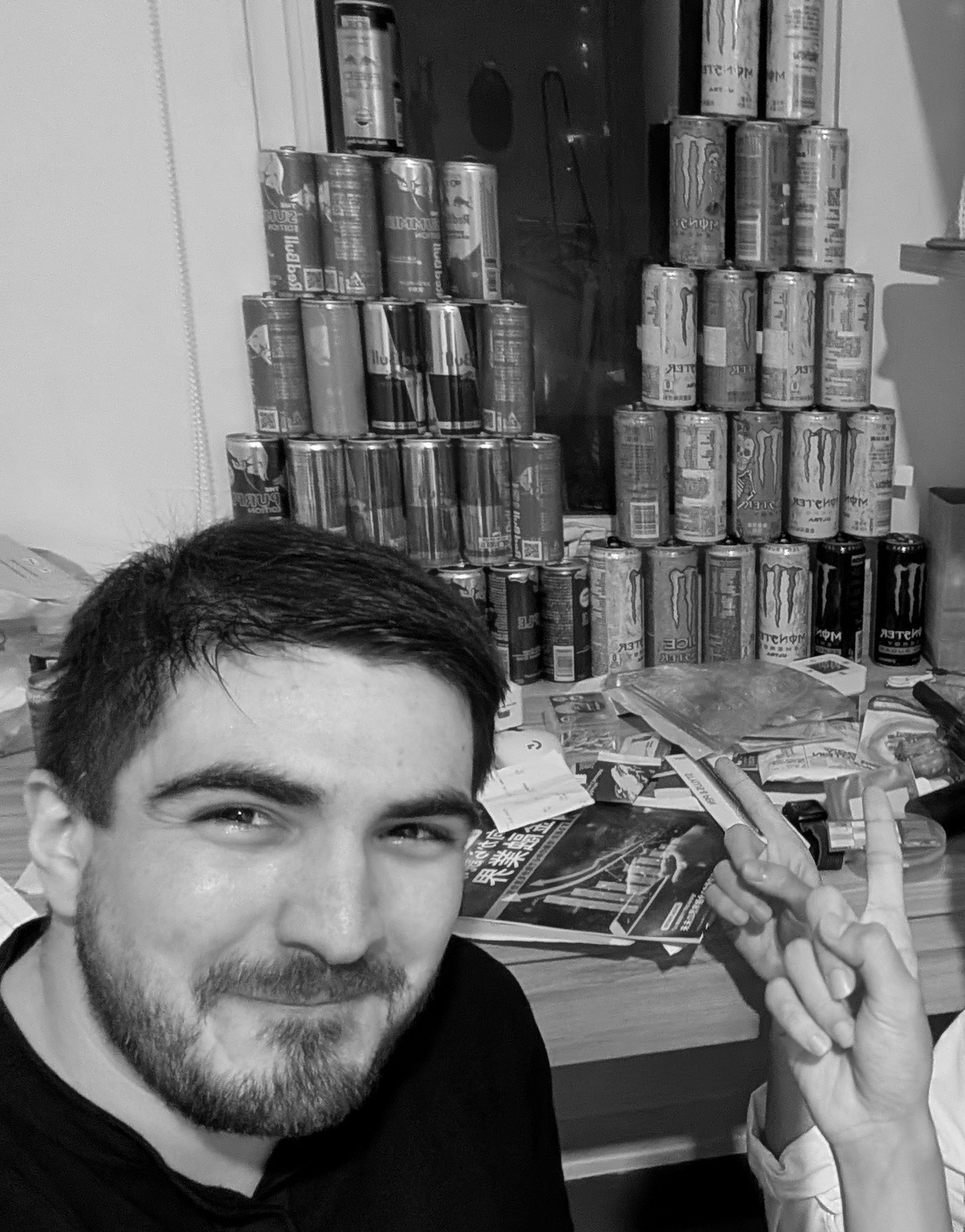
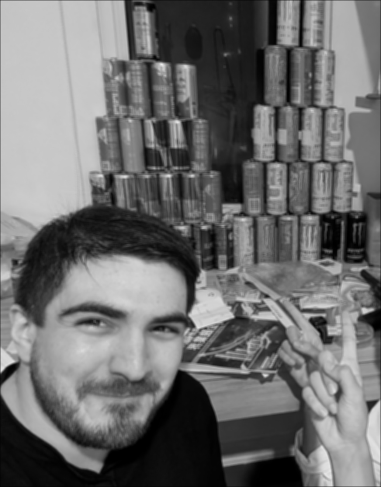
Zero fill treats everything outside the image as black. A 9×9 average near the border therefore mixes in up to half a window of zeros, and the edges darken: the mean intensity within 4 pixels of the border is 0.30 with zero fill versus 0.42 with reflection (boundary='symm'). The interior is identical in both cases (mean difference 1.2 × 10⁻¹⁶), since padding only affects pixels within the kernel radius of the edge. 'wrap' instead pulls in pixels from the opposite side of the image. For every part after 1.1, I use reflection, so the frame of the image never shows up as a fake edge.


symm). The border stays at the right brightness.
Selfie results
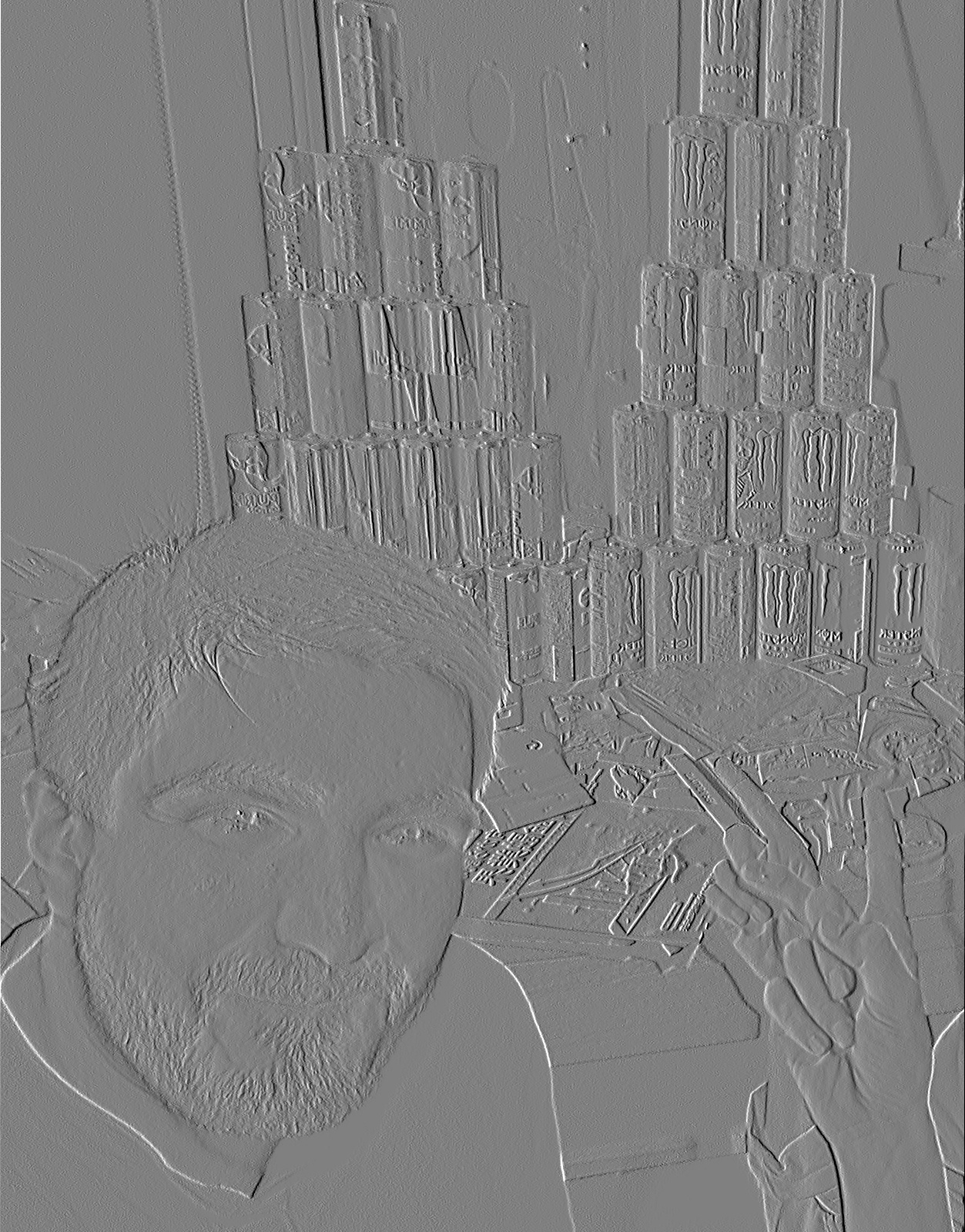
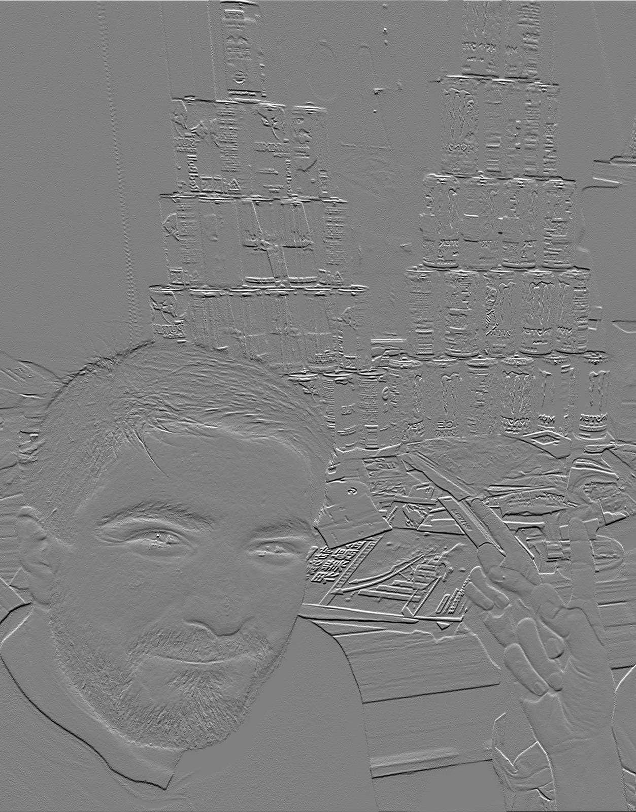
The timings above use a 376×480 copy, since the four-loop version would take minutes at full size. The figures below are computed at 1253×1600 with the tap-loop version, which produces identical output.
Part 1.2: Finite Difference Operator
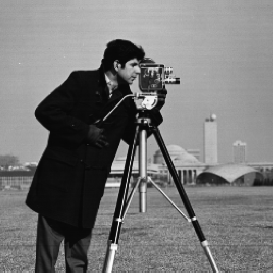
Convolving with \(D_x = [1, 0, -1]\) and \(D_y = D_x^\top\) gives a centered difference, \(I(x{+}1) - I(x{-}1)\), in each direction. Combining the two gives the gradient magnitude, which is large wherever intensity changes quickly in any direction:
The provided cameraman.png has a thin white margin (7 / 1 / 1 / 5 px on the top / bottom / left / right). I trim it before filtering; otherwise the frame of the image comes out as the strongest edge in the picture. The working image is 534×534.
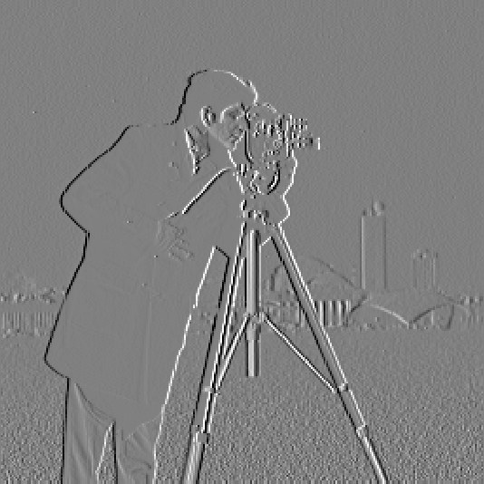
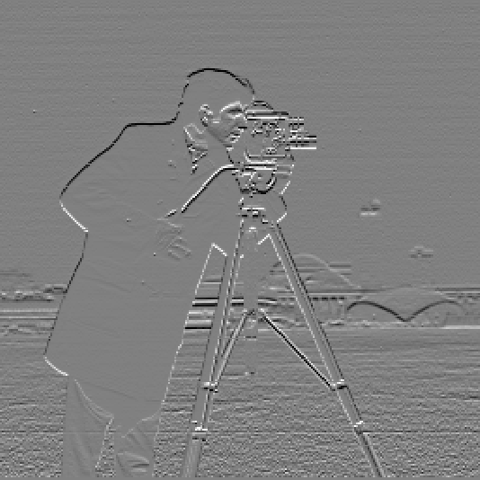
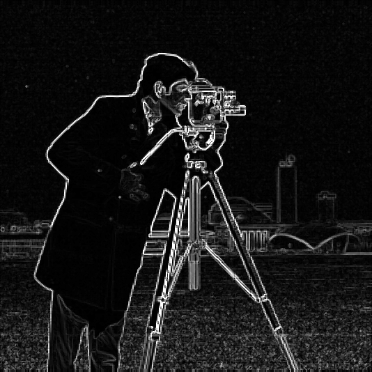
Choosing the threshold
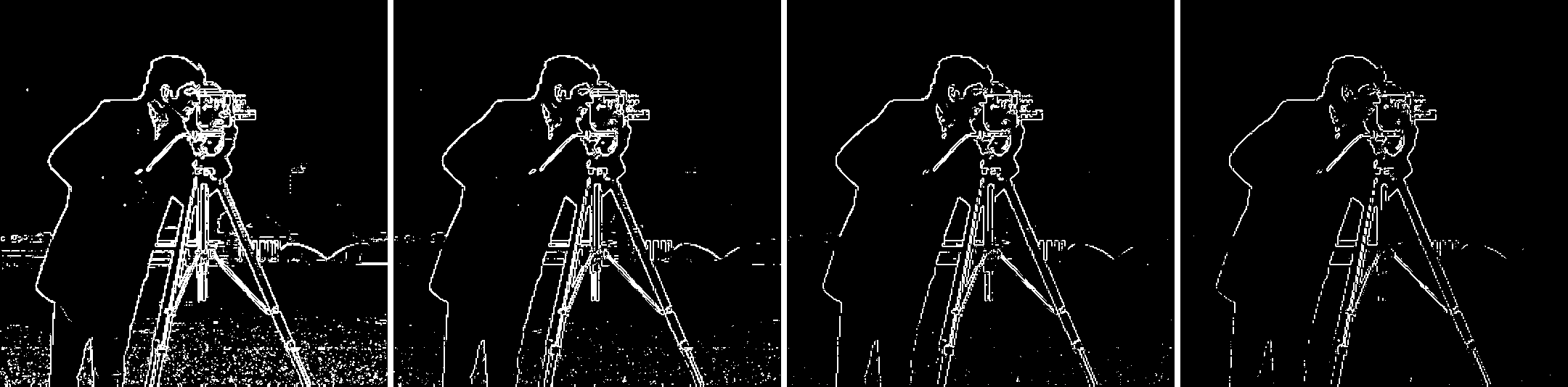
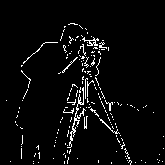
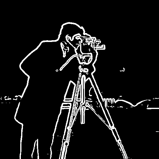
Binarizing trades two errors against each other: too low and the grass texture floods the image, too high and real edges break apart or disappear. I judged the threshold visually, as the assignment asks, and also counted connected edge blobs of four pixels or fewer as a rough measure of noise:
| Threshold | Edge pixels | Connected pieces | Blobs ≤ 4 px (noise) |
|---|---|---|---|
| 0.15 | 9.2% | 936 | 554 |
| 0.22 | 5.6% | 462 | 330 |
| 0.28 (chosen) | 4.1% | 305 | 170 |
| 0.35 | 2.9% | 370 | 183 |
The noise count is not monotone, which is the useful part. From 0.15 up to 0.28 it falls as the grass speckle drops out. Past 0.28 it climbs again (183 at 0.35) because the real edges start to fragment into short pieces, and the dome and buildings in the background disappear. I chose 0.28: it keeps the person, the camera, the full tripod, and most of the skyline, while accepting a few specks in the grass near the bottom.
Part 1.3: Derivative of Gaussian (DoG) Filter
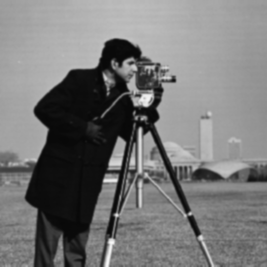
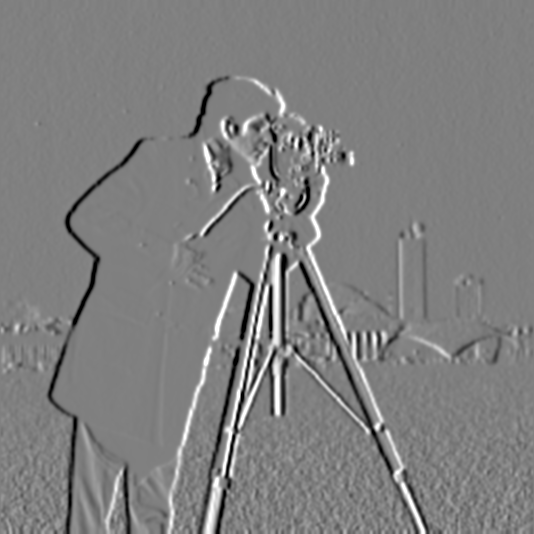
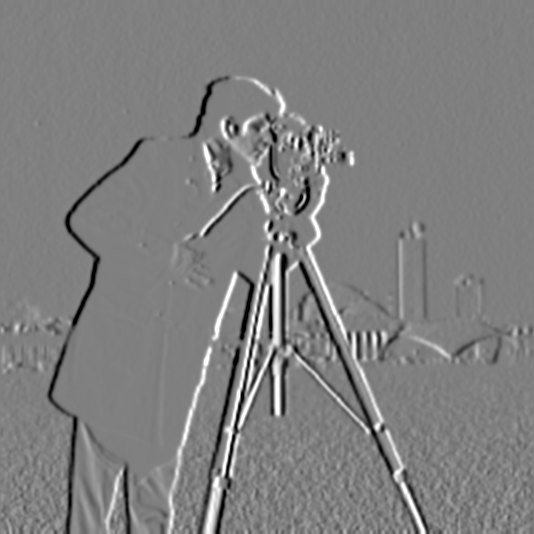
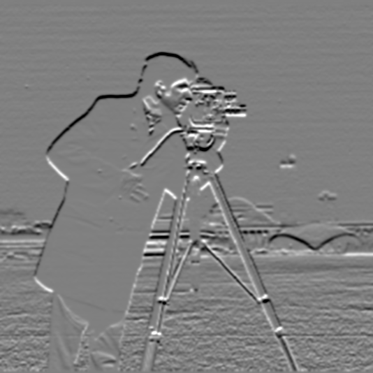
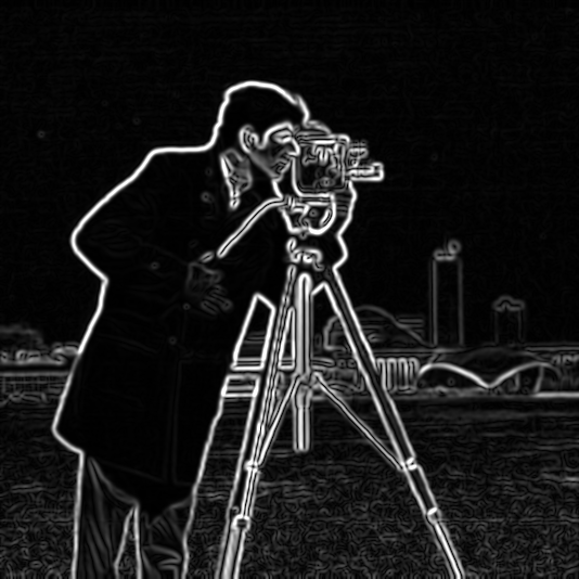
The finite difference only looks at two neighboring pixels, so it responds to pixel-level noise and texture as strongly as it responds to object boundaries. The fix is to low-pass first. I built a 1D Gaussian with cv2.getGaussianKernel(11, 1.5) (σ = 1.5, width 2⌈3σ⌉+1 = 11) and took its outer product with itself to get the 2D kernel \(G = g\,g^\top\), which sums to 1. Then I repeated the procedure above on the blurred image.
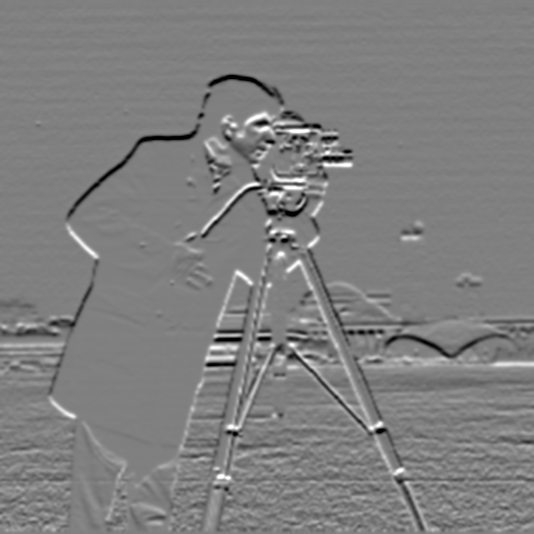
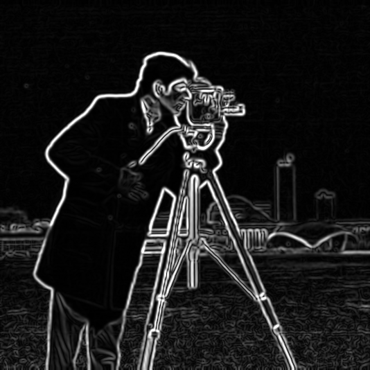
What changed
Three differences stand out compared with the plain finite difference:
- The noise is almost gone. At threshold 0.1 there are 20 tiny blobs, compared with 170 before (8.5× fewer), and the grass is clean.
- Edges are thicker and continuous. Blurring spreads each step over a few pixels, so the edges come out as smooth outlines instead of broken single-pixel lines. That is a loss of localization accuracy, and it's the trade you make for the noise reduction.
- The threshold has to change. Smoothing also lowers the peak derivative at every edge: the 99th percentile of the magnitude drops from 0.52 to 0.25. A threshold chosen for the raw image therefore does not carry over, and I re-picked it at 0.1.
One convolution instead of two
Convolution is associative, so \((I * G) * D_x = I * (G * D_x)\). Convolving the Gaussian with each difference operator once gives two 11×13 derivative-of-Gaussian (DoG) filters, and each can then be applied to the image in a single pass. Each DoG filter sums to 1.1 × 10⁻¹⁶, so it gives zero on a flat region, as a derivative filter should.
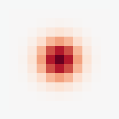
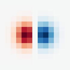
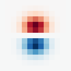
Verification. The DoG gradient magnitude matches the blur-then-differentiate result to within 1.1 × 10⁻¹⁵ over the entire image, borders included. The borders match as well because reflecting the image at its edges and then applying a symmetric Gaussian gives the same result as blurring first and then reflecting. As a second check, with zero padding and full output the two routes agree to 9.9 × 10⁻¹⁶.
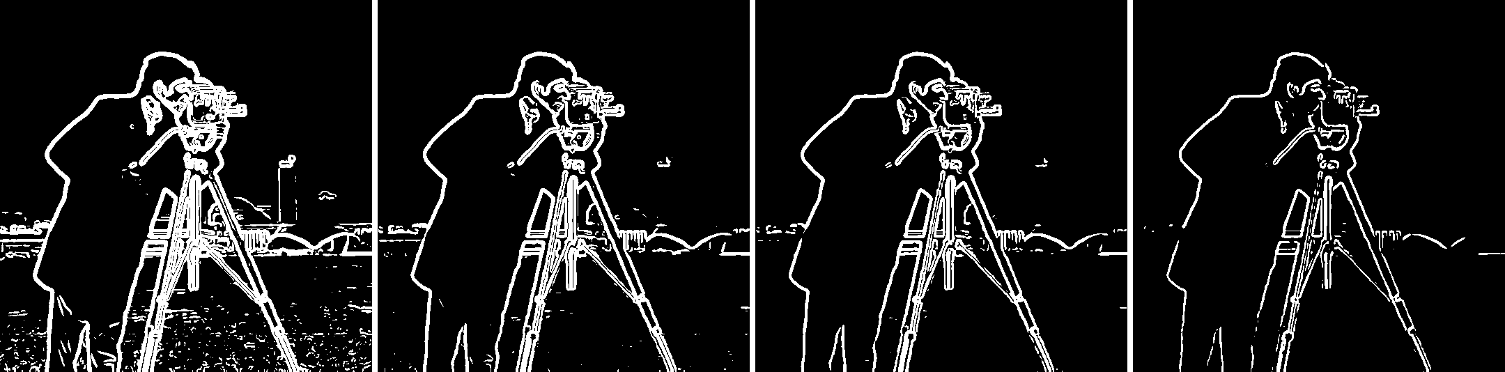
| DoG threshold | Edge pixels | Connected pieces | Blobs ≤ 4 px (noise) |
|---|---|---|---|
| 0.05 | 15.0% | 420 | 174 |
| 0.08 | 9.9% | 125 | 54 |
| 0.1 (chosen) | 8.1% | 85 | 20 |
| 0.15 | 5.0% | 117 | 28 |
Part 1 Bells & Whistles: Gradient Orientation
The gradient direction is \(\theta = \operatorname{atan2}(g_y, g_x)\), taken here from the DoG responses so that the noise doesn't turn into random colors. The assignment asks for this without built-in angle functions, so I wrote my own atan2:
- Reduce to one octant. Using \(|g_x|\) and \(|g_y|\), take \(z = \min/\max\), which is always in \([0, 1]\).
- Evaluate arctan on [0, 1] with a polynomial. This is the Abramowitz & Stegun 4.4.49 approximation, \(\arctan z \approx z(0.99987 - 0.33030z^2 + 0.18014z^4 - 0.08513z^6 + 0.02084z^8)\).
- Undo the reduction. Apply \(\pi/2 - a\) if \(|g_y| > |g_x|\), \(\pi - a\) if \(g_x < 0\), and negate if \(g_y < 0\).
Compared against np.arctan2, which I used only for this check, the maximum error over all 534×534 pixels is 1.1 × 10⁻⁵ rad (mean 7.2 × 10⁻⁶), far below anything visible in a color map. For the visualization, hue encodes the direction \(\theta / 2\pi\), saturation is 1, and value is the gradient magnitude normalized by its 99th percentile, so flat regions stay dark instead of showing random hue. The color wheel on the right is produced by the same code, fed a synthetic gradient field that points outward in every direction. Image \(y\) points down, so angles increase clockwise.
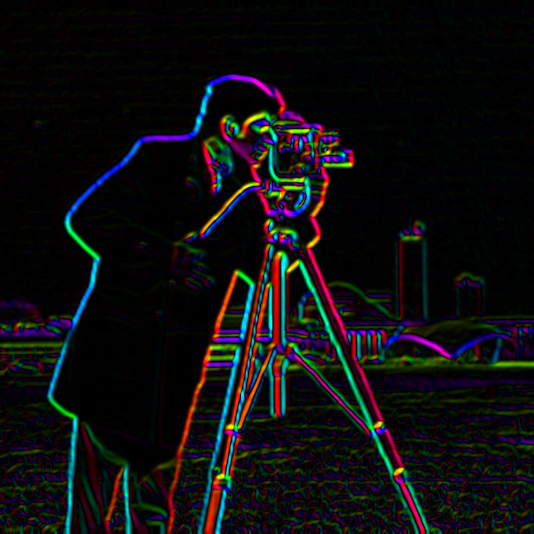
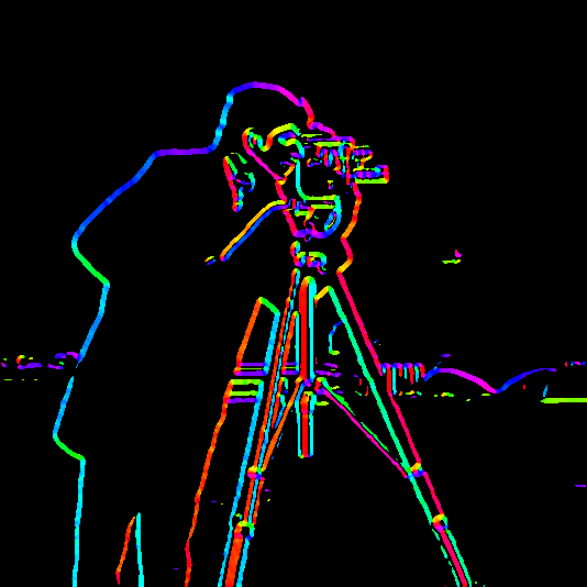
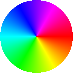
Two things are easy to read from this map. First, the two sides of a thin dark object get opposite hues. Each tripod leg is red on one side and cyan on the other, because the gradient always points from dark to bright. Second, the scene is dominated by vertical structure: 58% of the edge gradient energy (weighted by magnitude) is within 30° of horizontal, meaning it comes from near-vertical edges such as the legs, coat and buildings. Only 19% comes from near-horizontal edges.
Fun with Frequencies!
Using the same filters as tools: sharpening, hybrid images, and multiresolution blending.
Part 2.1: Image “Sharpening”
A Gaussian is a low-pass filter, so \(f * G\) keeps only the slow variations in the image. Subtracting that from the original leaves exactly what the blur removed: the high frequencies, \(f - f * G\). Photographs look sharper when those are stronger, so unsharp masking adds a scaled copy of them back. Because everything involved is linear, the whole operation collapses into one convolution:
Here \(e\) is the unit impulse, the filter that leaves an image unchanged. The resulting kernel is a positive spike at the center surrounded by a shallow negative Gaussian. I use σ = 2.0 (13×13 kernel) and apply it per color channel. The single-filter result matches the two-step version to within 1.7 × 10⁻¹⁵.
def unsharp_kernel(sigma, alpha, ksize=None):
    G = gaussian_2d(sigma, ksize)
    e = np.zeros_like(G)
    e[G.shape[0] // 2, G.shape[1] // 2] = 1.0
    return (1 + alpha) * e - alpha * G
Taj Mahal
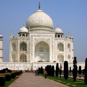
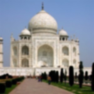
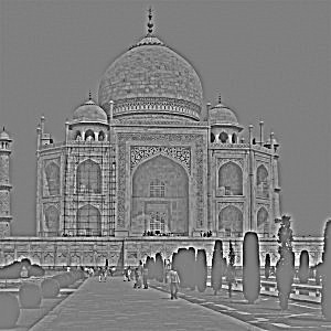
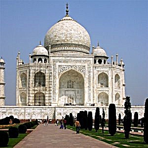
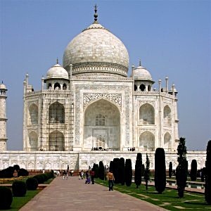
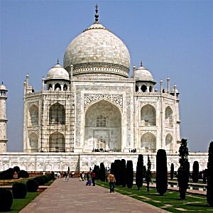
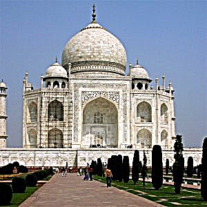
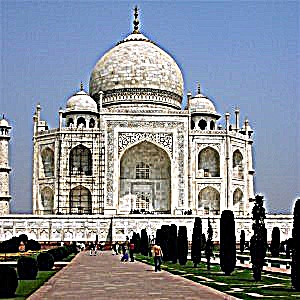
I measure sharpness as the mean gradient magnitude of the luminance. At α = 1.5 it goes from 0.080 to 0.157 (2.0×). Increasing α keeps raising that number, but past about α = 2 the extra gain shows up as bright and dark halos along every edge, and the white marble facade blows out to pure white. A higher sharpness number does not mean a better-looking image.
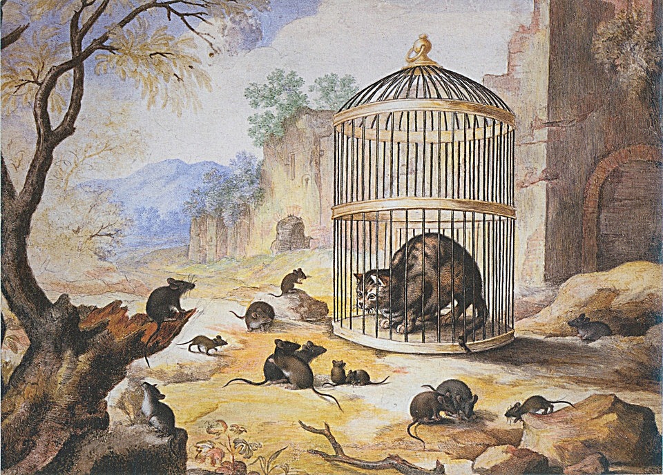
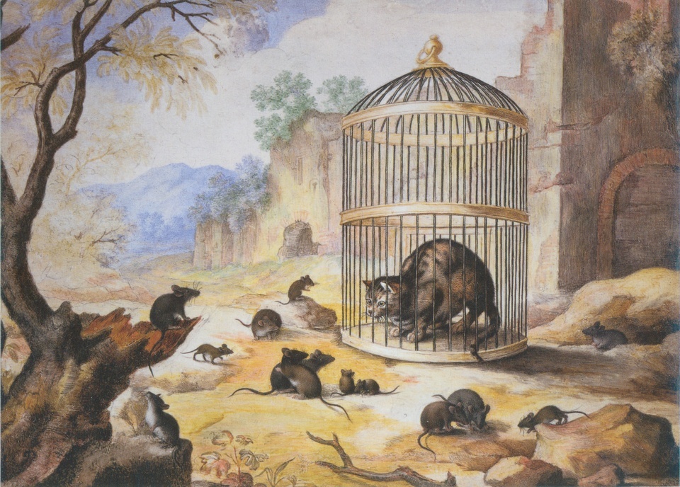
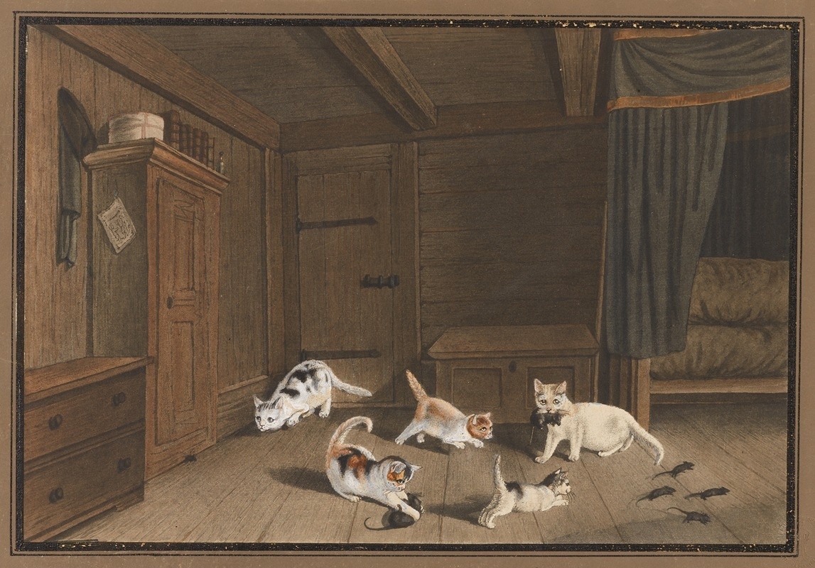
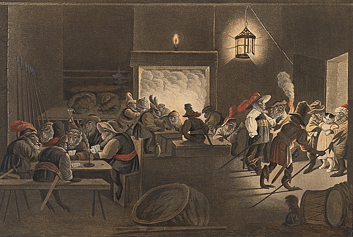
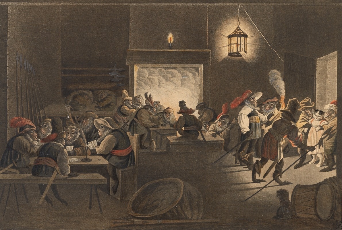
My picks: three paintings by Gottfried Mind
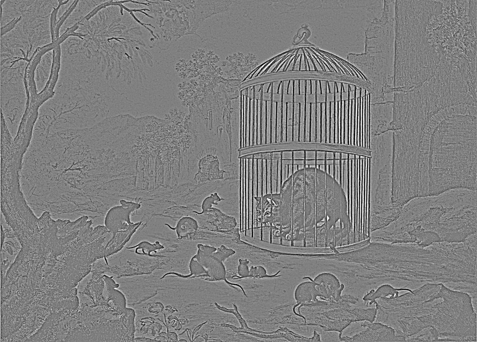
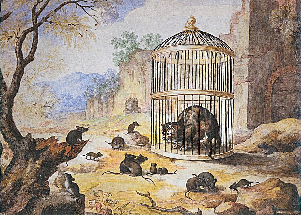
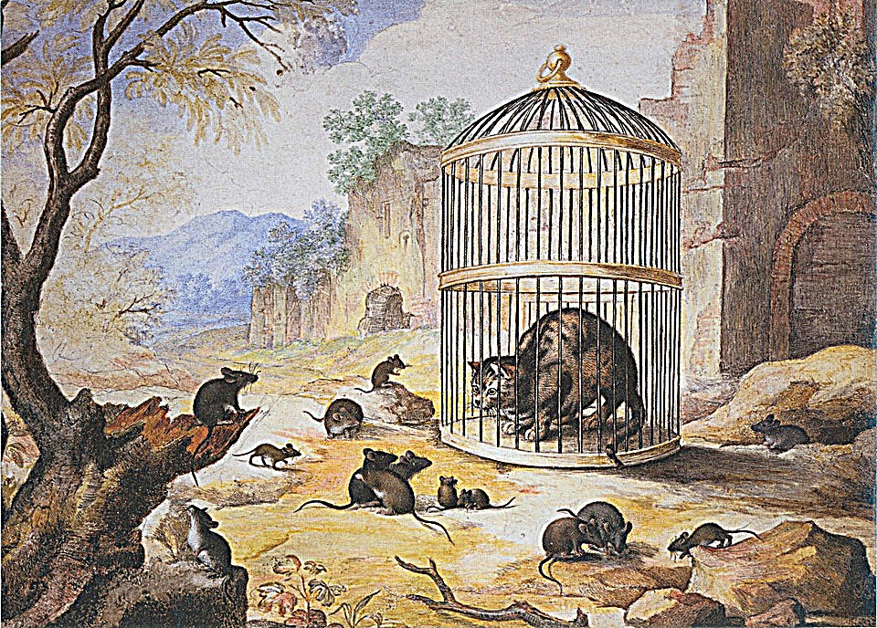
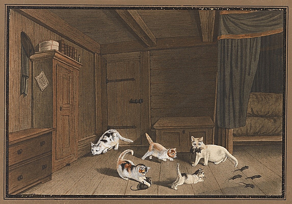
For my own images I chose scans of three paintings by Gottfried Mind, the Swiss painter known for his cats. Old scans are soft, which makes them natural candidates for sharpening. At α = 1.5, sharpness rises by 2.2× to 2.3×. The fur strokes, cage bars and furniture edges come back clearly, but so does the paper grain, because the filter cannot tell texture from noise. The paintings also clip far less than the Taj at α = 4 (10% vs. 23% of values), since they are mostly mid-tones with few near-white areas to blow out.
Evaluation: blur a sharp photo, then try to undo it
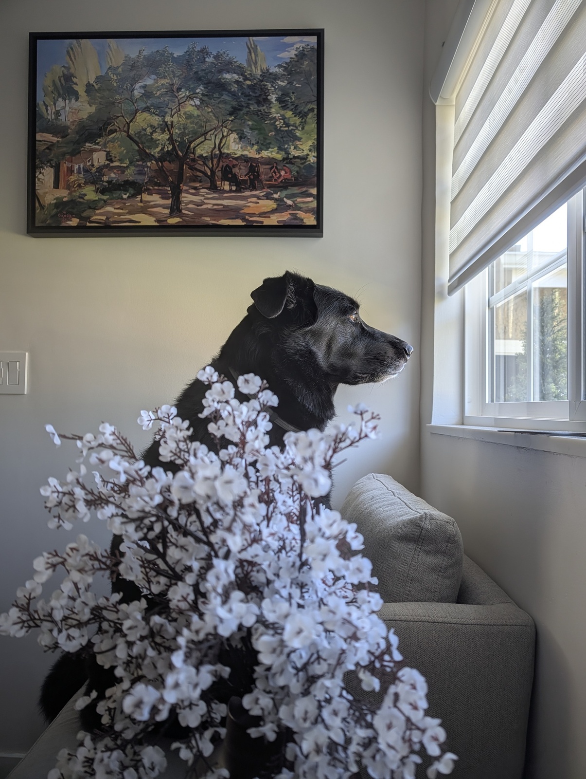
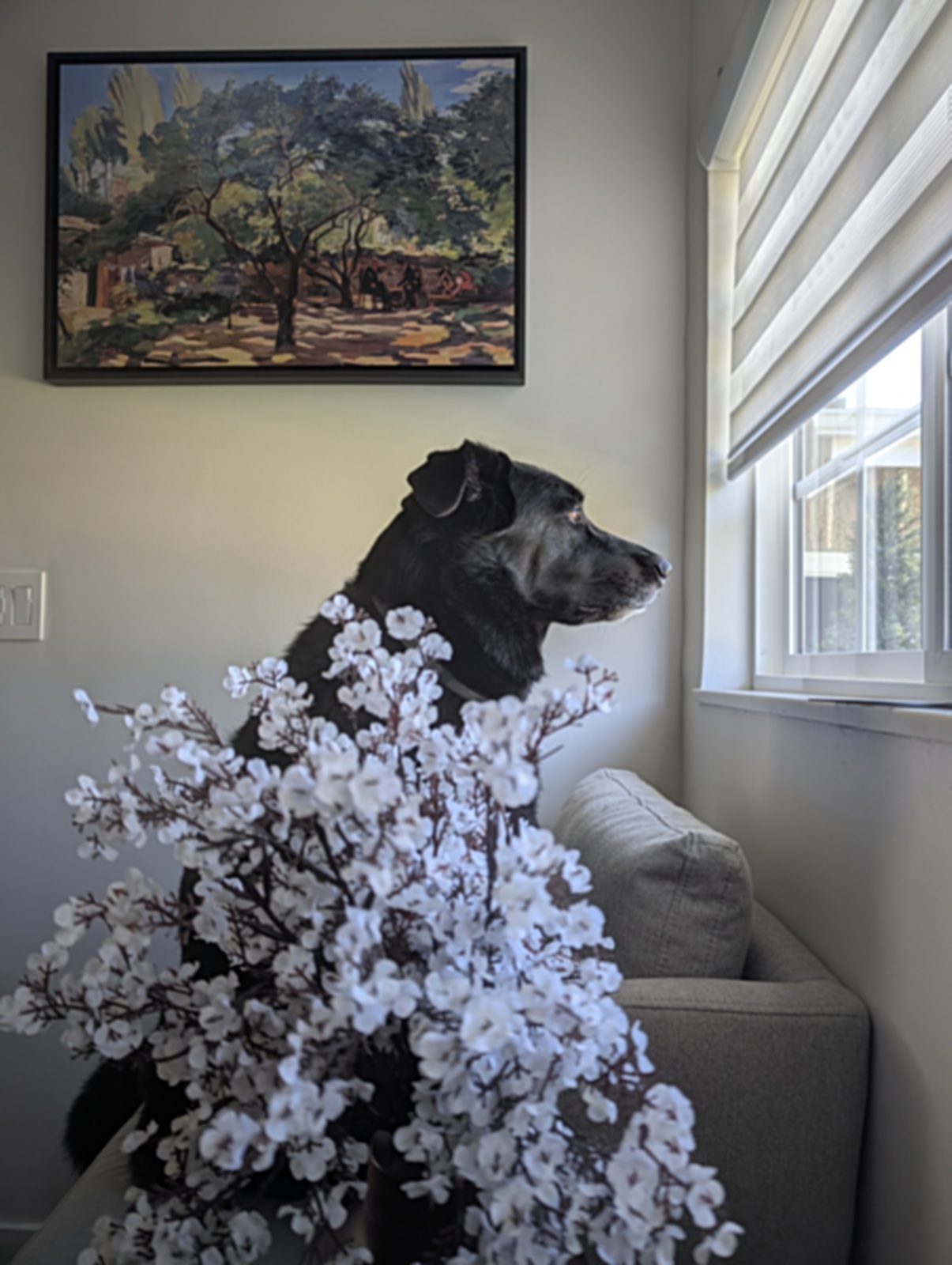
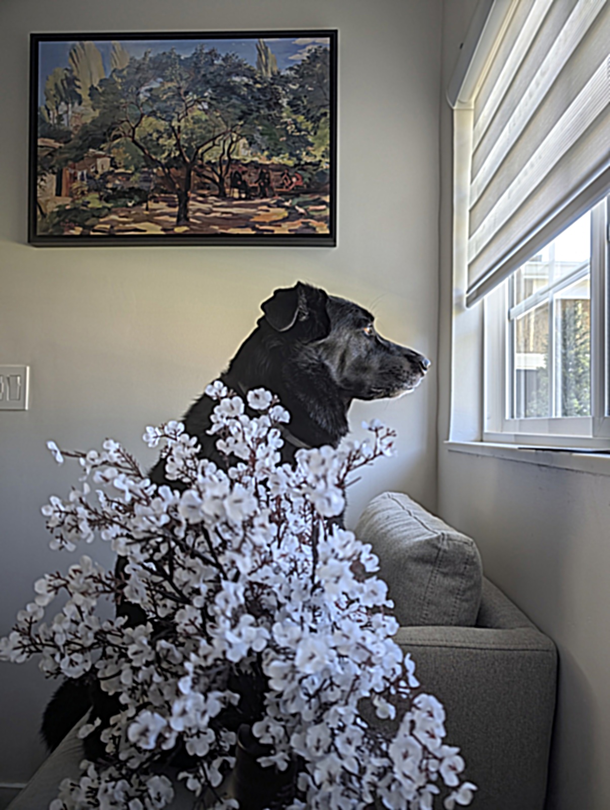
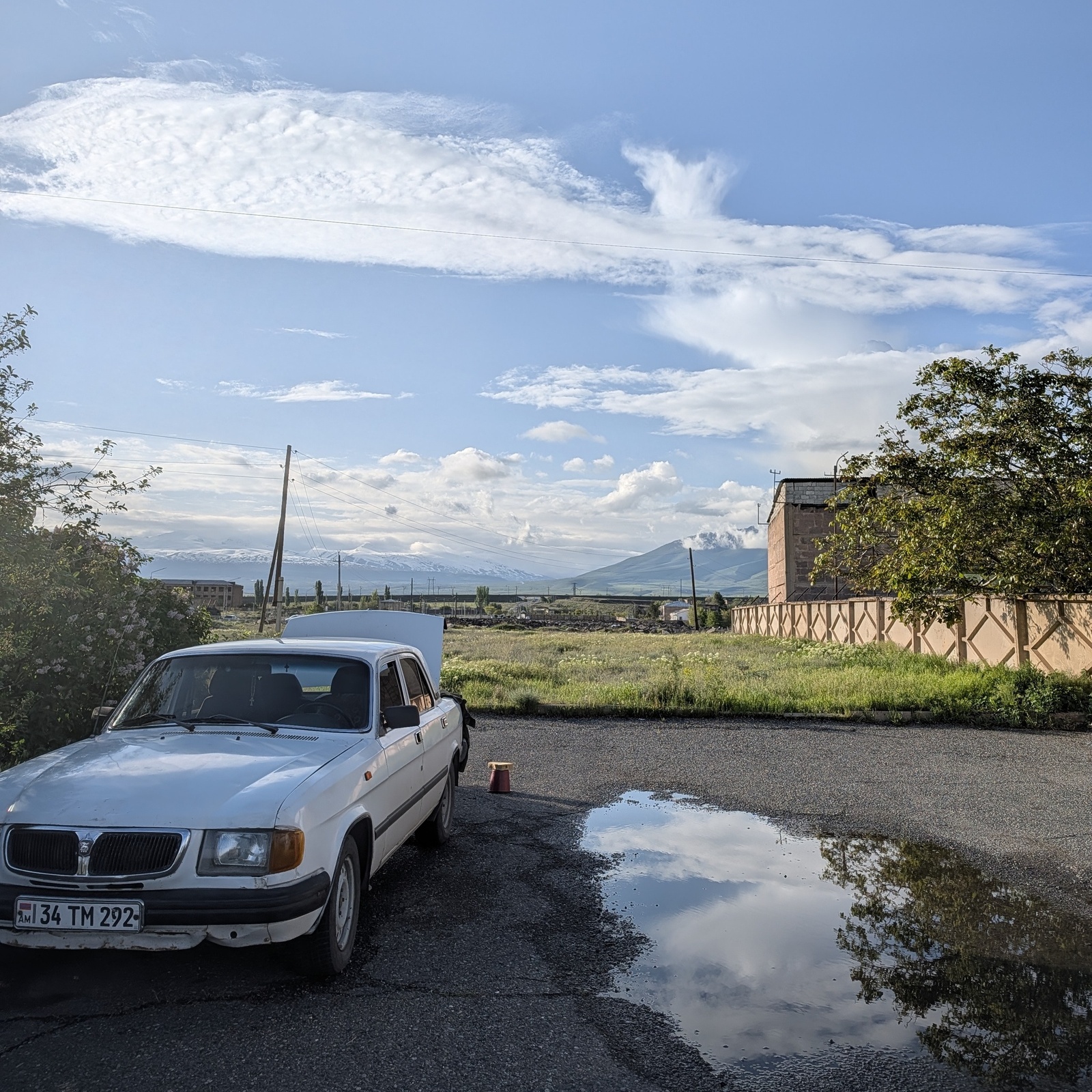
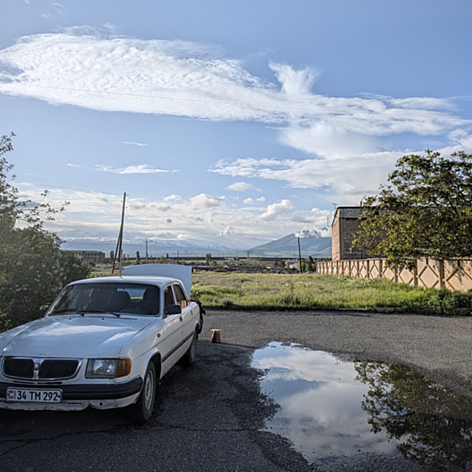
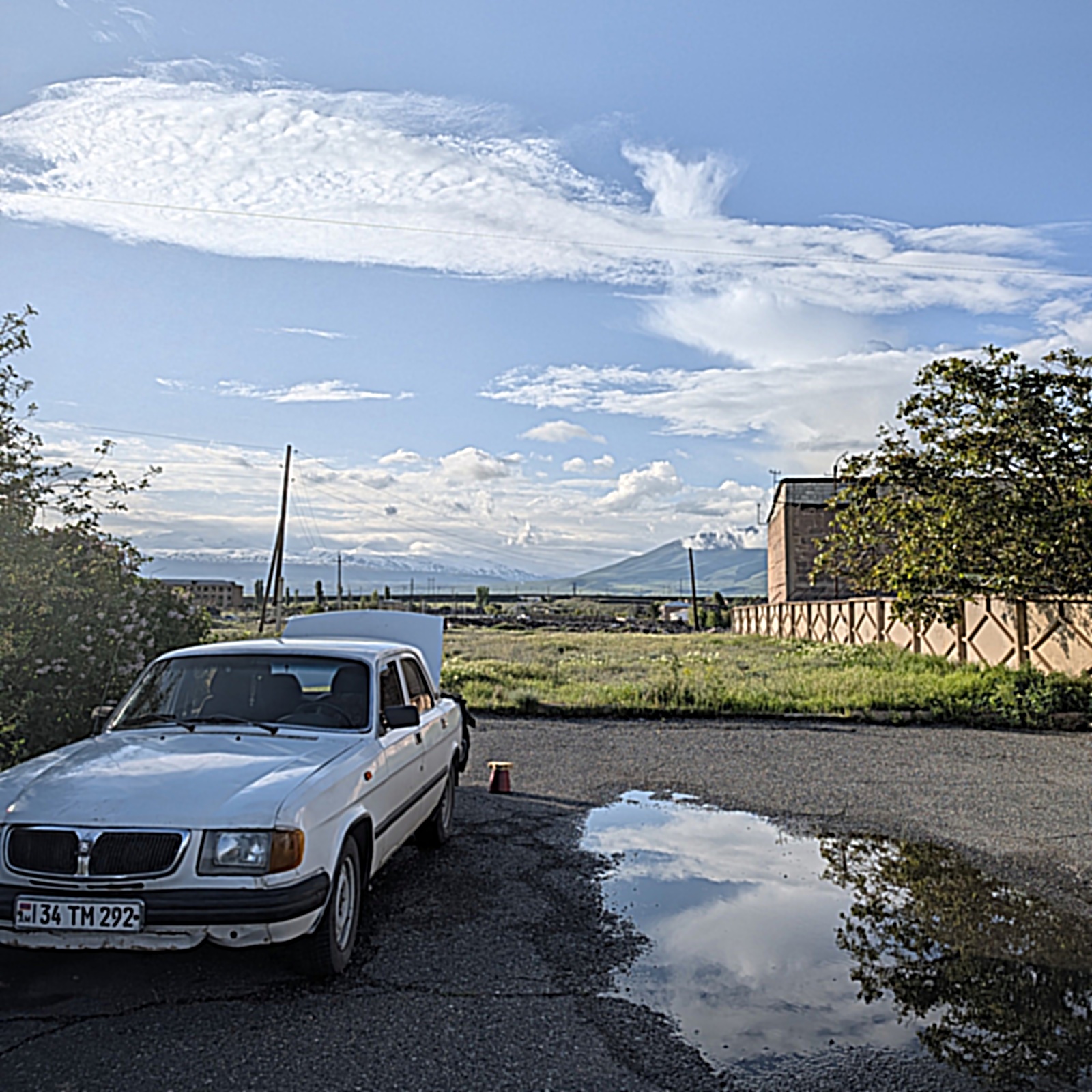
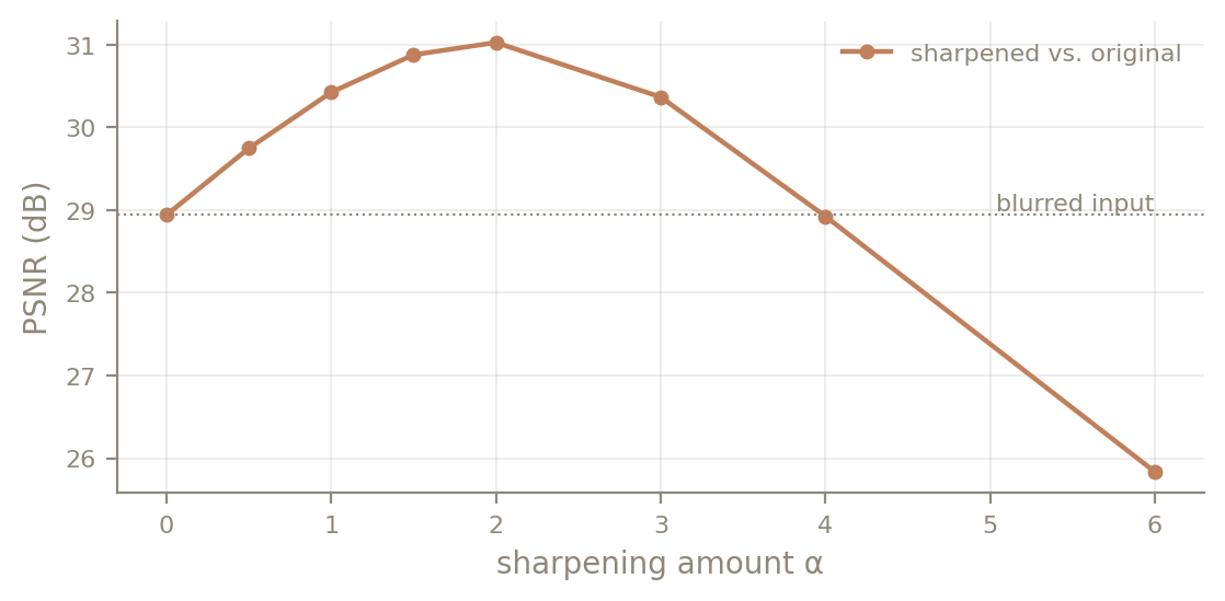
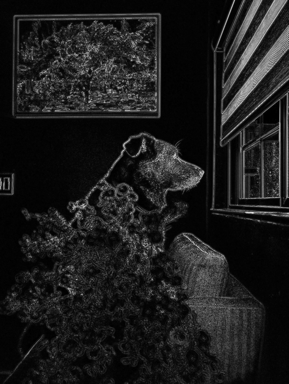
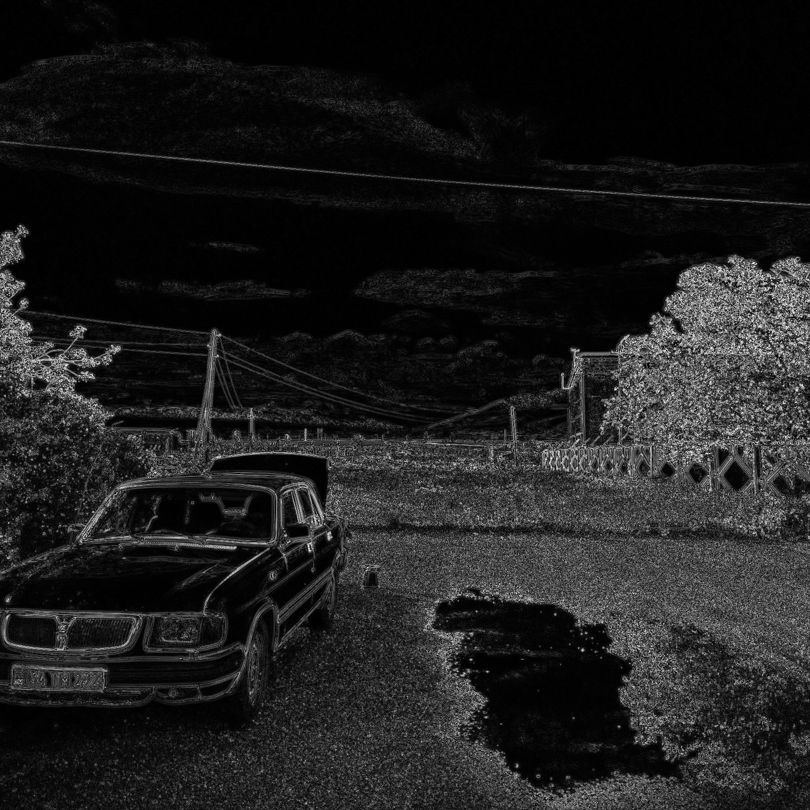
To see what sharpening can and cannot do, I took two crisp phone photos of my own: my dog, and a car next to a puddle. I blurred each with σ = 2.0, sharpened the blurred copy with the same σ over a range of α values, and scored every result against the original with PSNR (higher means closer to the original).
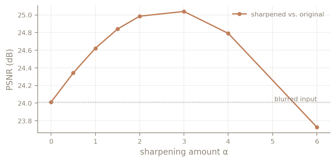
| α | Dog PSNR | Dog sharpness | Car PSNR | Car sharpness |
|---|---|---|---|---|
| 0 | 28.94 dB | 0.022 | 24.01 dB | 0.018 |
| 0.5 | 29.75 dB | 0.024 | 24.34 dB | 0.021 |
| 1 | 30.43 dB | 0.026 | 24.62 dB | 0.024 |
| 1.5 | 30.88 dB | 0.029 | 24.84 dB | 0.028 |
| 2 | 31.03 dB | 0.032 | 24.99 dB | 0.031 |
| 3 | 30.37 dB | 0.037 | 25.04 dB | 0.038 |
| 4 | 28.93 dB | 0.043 | 24.79 dB | 0.045 |
| 6 | 25.84 dB | 0.054 | 23.73 dB | 0.057 |
Sharpening helps, but only partly, and how much depends on the photo. For the dog, the best setting (α = 2) recovers 2.08 dB. For the car it recovers only 1.03 dB, even at its best α = 3. The car photo is mostly fine texture: gravel, grass and distant trees. The σ = 2.0 blur attenuates nearly all of that, so there is little left to amplify, and the remaining error covers the whole frame instead of just the edges. Over-sharpening fails the same way on both: at α = 6 the dog's measured sharpness (0.054) is higher than the original's (0.048), yet PSNR falls below even the blurred input. The extra contrast is halos and amplified noise, not detail recovered from the blur.
Part 2.2: Hybrid Images
A hybrid image (Oliva, Torralba & Schyns, 2006) keeps the low frequencies of one image and the high frequencies of another:
Up close, the eye picks up the fine edges of \(I_2\). From far away, or when the image is small, those edges are too fine to resolve and only the blurry structure of \(I_1\) remains. Following the paper, I define each filter's cutoff as the frequency where its gain is ½. A Gaussian with standard deviation σ has gain \(e^{-2\pi^2\sigma^2 f^2}\), which is ½ at
I specify the cutoffs in cycles per image over the shorter side \(N\), rather than as σ in pixels, because my aligned pairs range from 421 to 1000 pixels wide. That way the same setting produces the same effect regardless of resolution. A cycle is one bright-and-dark stripe pair, so for example "6 cycles/image" keeps only structure coarse enough that six stripe pairs would span the image.
def hybrid_image(im_low, im_high, sigma_low, sigma_high, color='both', gain_high=1.0):
    low_src = im_low if color in ('both', 'low') else to_gray(im_low)
    high_src = im_high if color in ('both', 'high') else to_gray(im_high)
    low, high = split_bands(low_src, high_src, sigma_low, sigma_high)
    if low.ndim != high.ndim:
        low, high = as_rgb(low), as_rgb(high)
    hyb = low + gain_high * high
    return np.clip(hyb, 0, 1), low, high
Alignment
Alignment builds on the provided starter code, with three changes:
- Saved points. Corresponding points live in
points/*.jsoninstead of being clicked on every run, so the results are reproducible. - No lost resolution. The starter always shrinks whichever image has its points farther apart. I resize the warped image first, so the reference image keeps its native resolution. For a hybrid the reference is the high-frequency image, whose fine detail is the whole point; the low-frequency image is about to be blurred anyway.
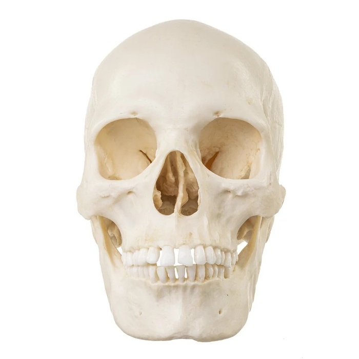
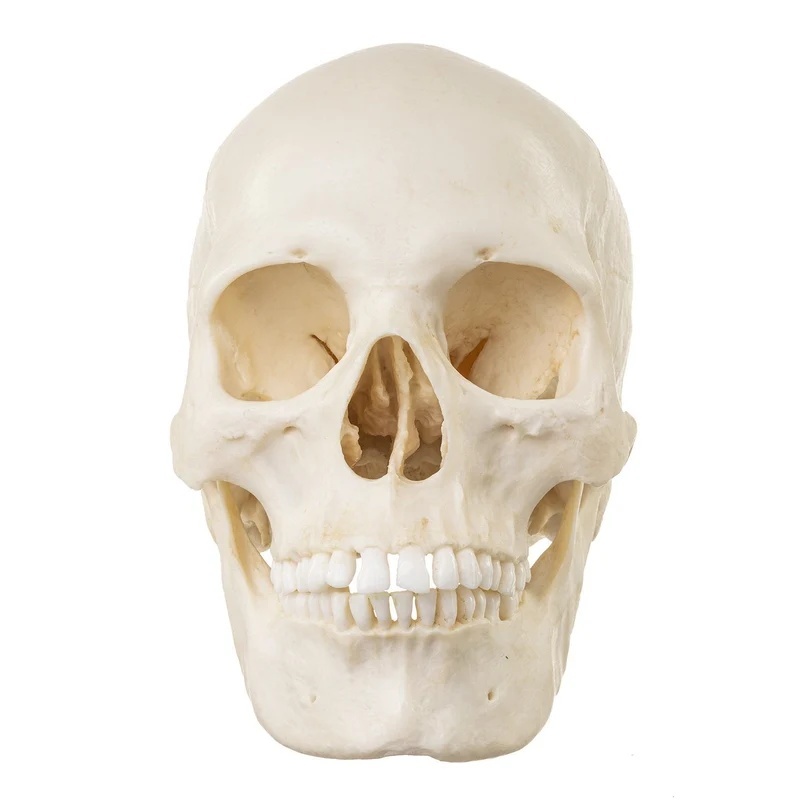
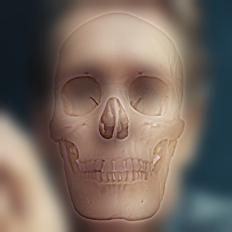
- Three points, affine warp. Derek + Nutmeg uses the starter's two-point similarity transform on the eyes. My pairs use three points (both eyes plus the mouth) and solve an affine transform, which can also stretch and shear. The paper itself suggests an affine warp for misaligned faces, and two points simply cannot put a skull's teeth on a mouth. The bear skull is fitted cheek to cheek with its nasal opening on the nose, because a bear's eye sockets sit far out on the sides of the skull.
The paper recommends warping the image that ends up in the low frequencies, and I do that throughout. After warping, I crop to the largest rectangle that is valid in both images, so no padding reaches the result.
| Hybrid | Low (far) | High (close) | Alignment | Size | Cutoff low / high (c/i) | High gain |
|---|---|---|---|---|---|---|
| Derek + Nutmeg | Derek | Nutmeg | starter, 2 pts | 516×772 | 10 / 16 | 1 |
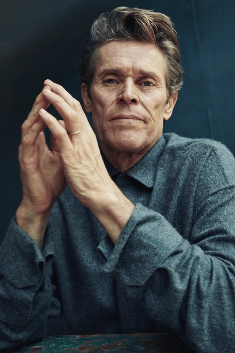
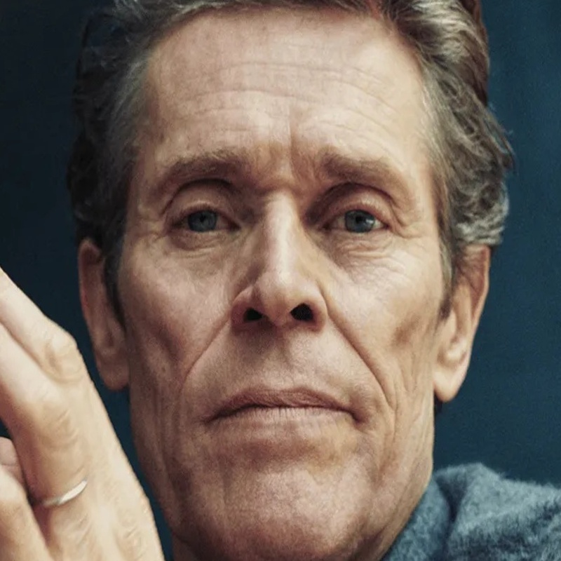
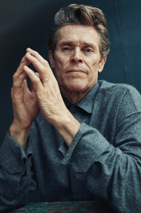
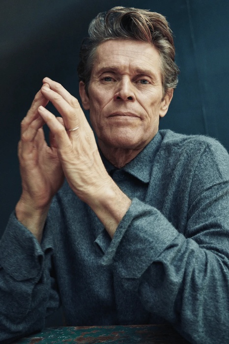
| Dafoe + skull | Dafoe, calm | human skull | affine, 3 pts | 800×800 | 6 / 24 | 1 |
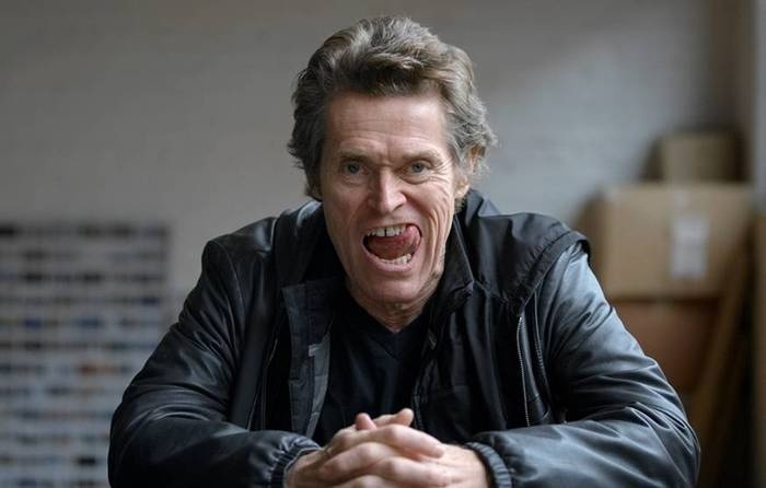
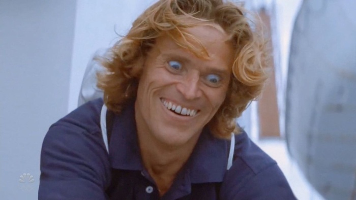
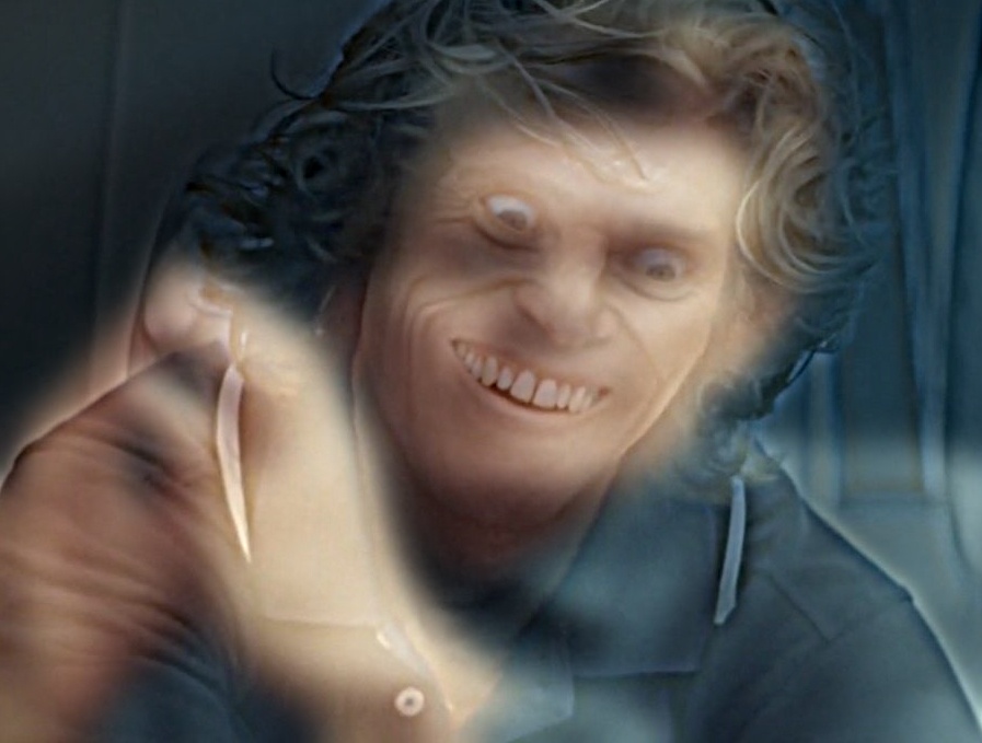
| Calm + manic Dafoe | Dafoe, calm | Dafoe, manic | affine, 3 pts | 421×373 | 8 / 14 | 1 |
| Calm + wild Dafoe | Dafoe, calm | Dafoe, SNL grin | affine, 3 pts | 897×679 | 8 / 16 | 1 |
| Chimp + skull | chimpanzee | chimpanzee skull | affine, 3 pts | 1000×880 | 16 / 28 | 0.8 |
| Bear + skull | brown bear | bear skull | affine, 3 pts | 922×882 | 16 / 28 | 0.8 |
Favorite: Dafoe + skull, full process
Which image goes in which band is not arbitrary. A skull on a white background is a strong, symmetric, high-contrast shape: bright bone with two dark sockets. If it were the low-frequency image, that shape would stay visible even up close, which is exactly the grouping problem the paper warns about. As the high-frequency image, all that survives is its edges (teeth, sutures, the rims of the sockets), and the white background high-passes to zero, so Dafoe's own dark backdrop shows through. Dafoe's face supplies the soft shading that the skull's edges sit on.
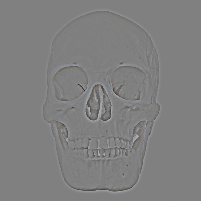
Frequency analysis
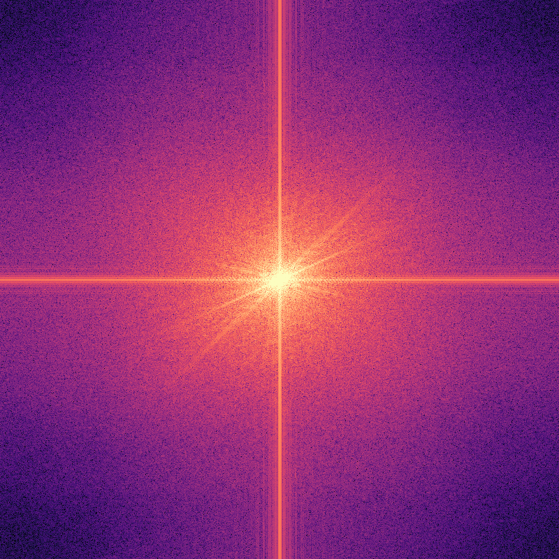
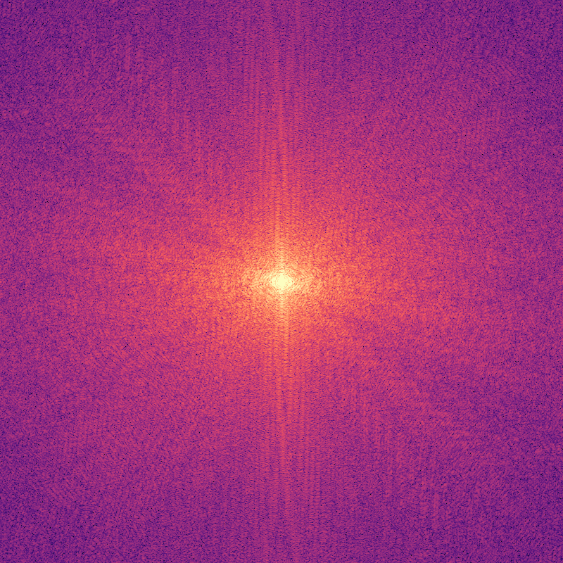
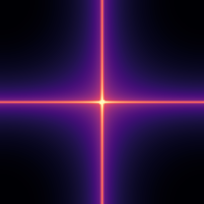
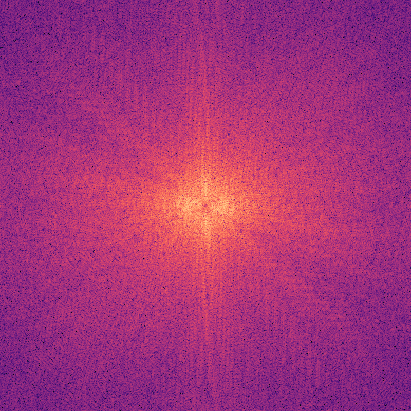
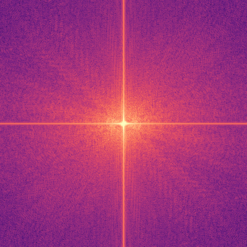
These are the log magnitudes of the 2D Fourier transforms, \(\log\lvert\mathcal{F}\{I\}\rvert\), with zero frequency at the center. All five share one color scale, so brightness can be compared across panels. The low-pass keeps only a small bright core, and everything outside it drops toward black. The high-pass does the reverse: it removes the core and keeps the surrounding texture. The hybrid's spectrum has both, with the portrait's core in the middle and the skull's energy around it.
Choosing the cutoffs
The paper's Figure 5 argues for leaving a gap between the two filters, and trying three settings on the same pair shows why. Each plot shows the gain of both filters for that setting:
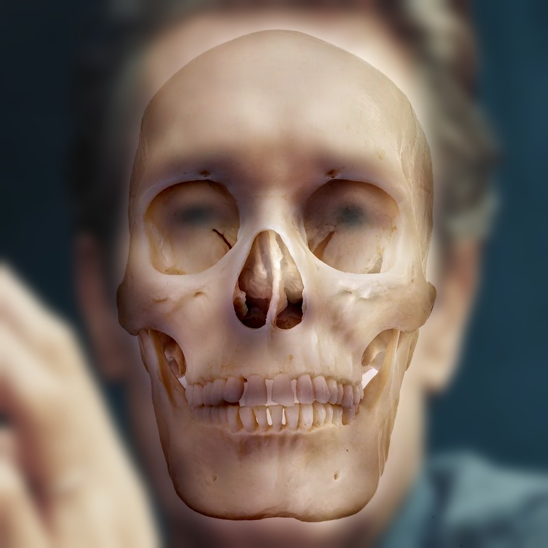
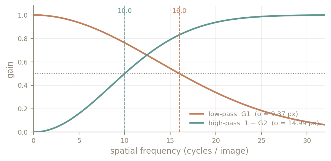
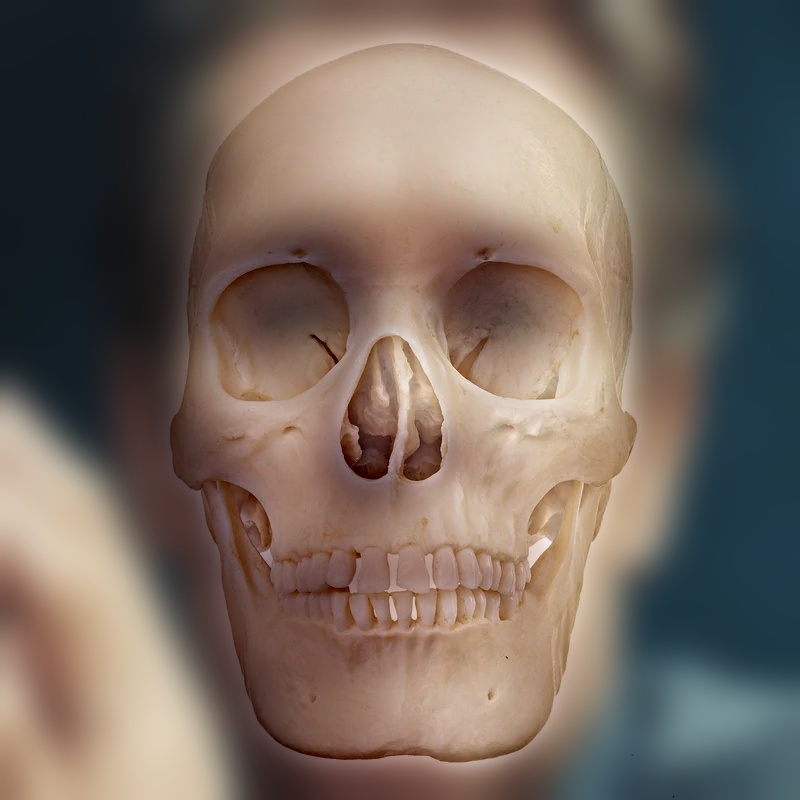
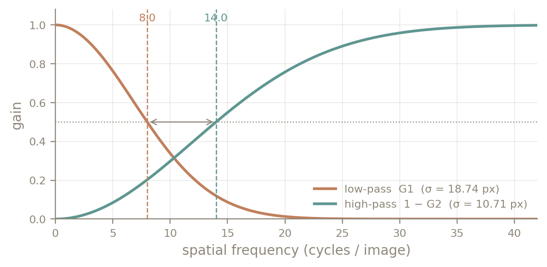
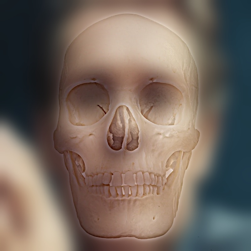
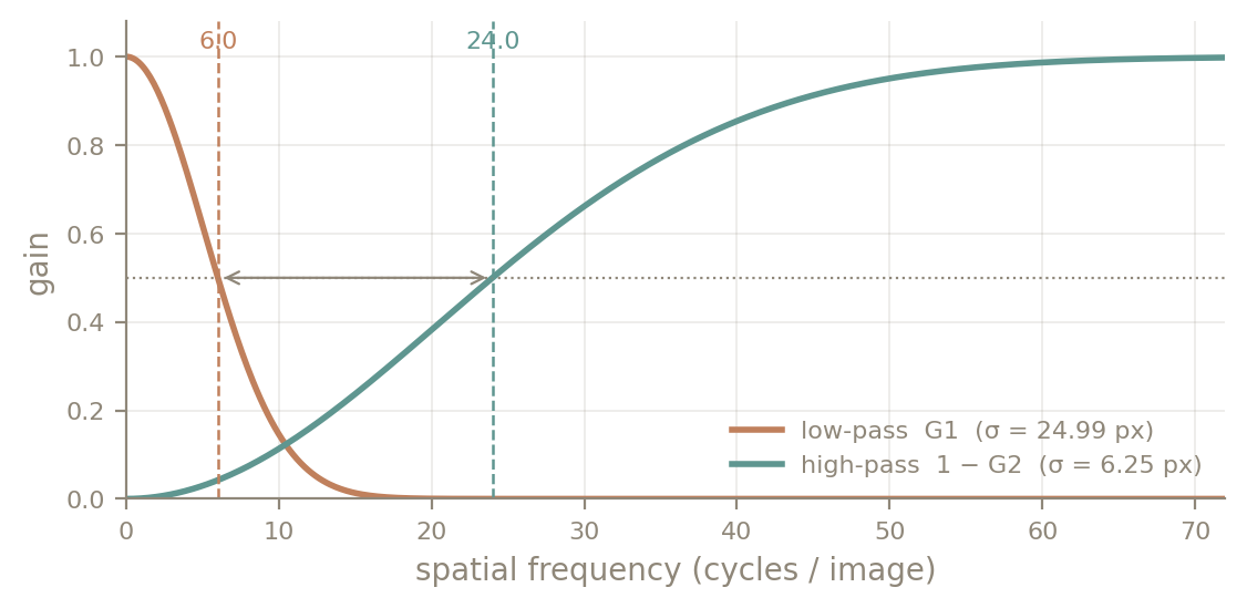
With the cutoffs crossed, both faces share the same frequency band and read as a double exposure at every distance. A narrow gap is almost there, but the teeth and eye sockets are mid-frequency features with strong contrast, and they still show through from far away. Moving the high cutoff up to 24 c/i and the low cutoff down to 6 c/i gives the skull only its finest edges and the portrait only its coarsest shading. At that point the switch happens cleanly as you step back.
Result
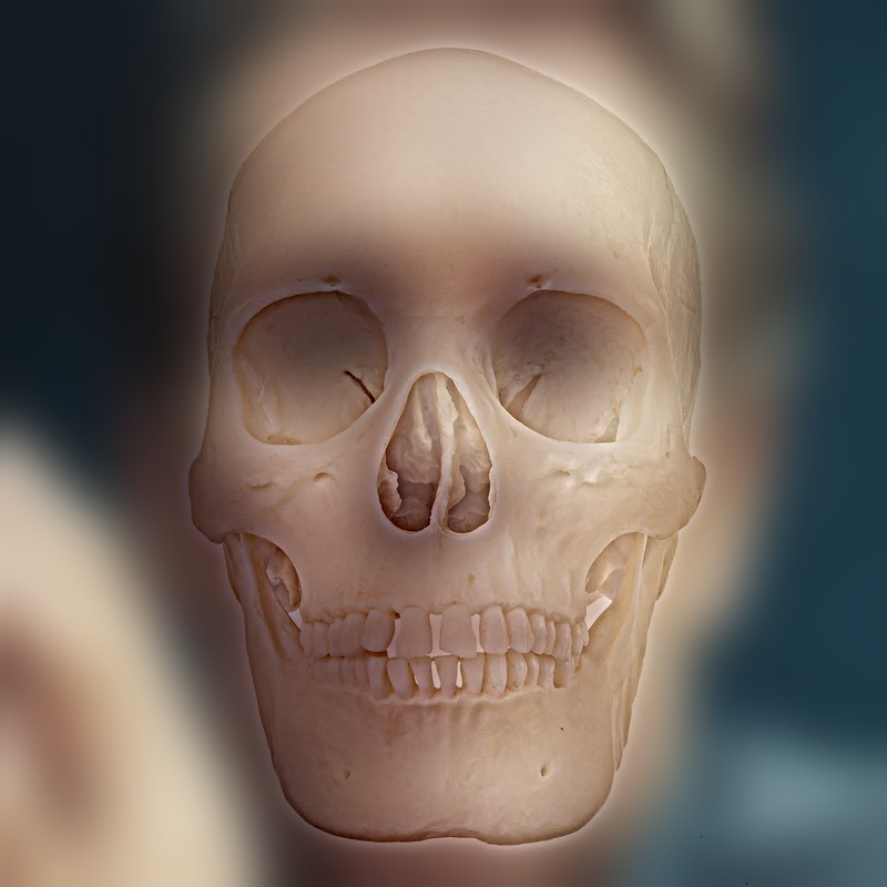
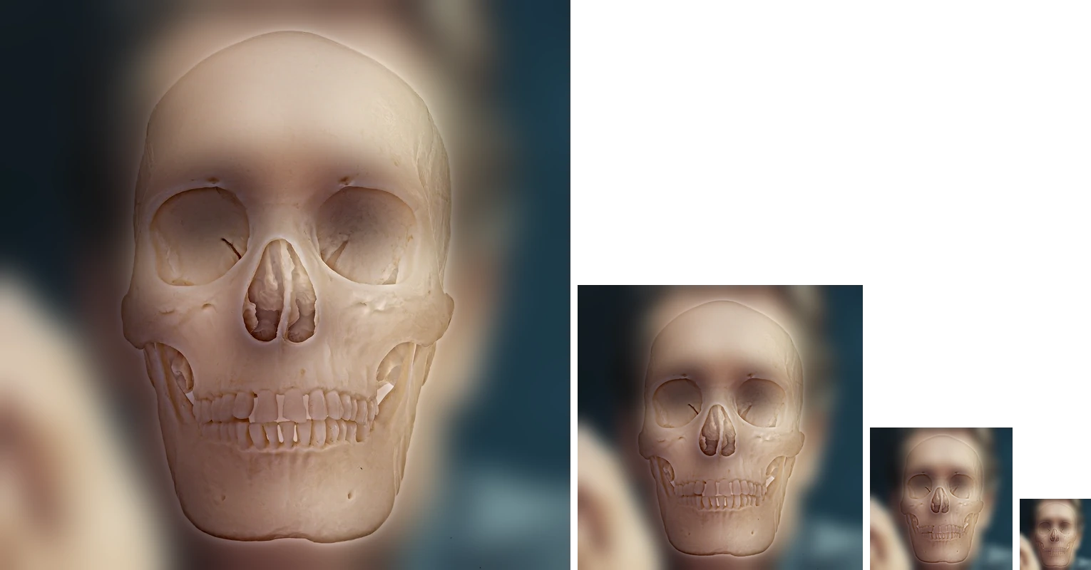
More hybrids
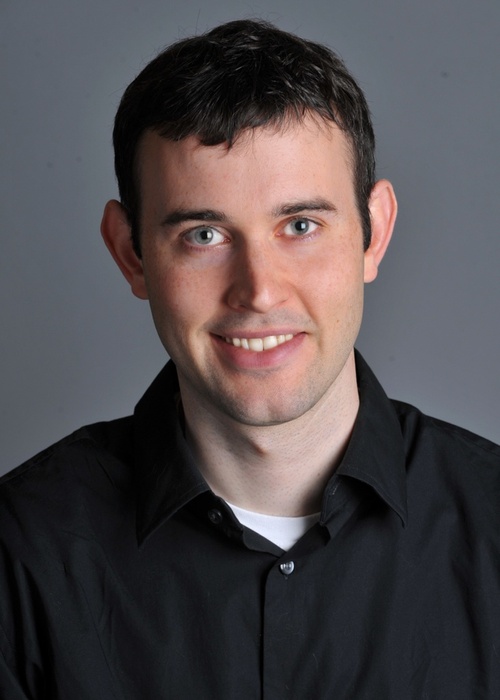
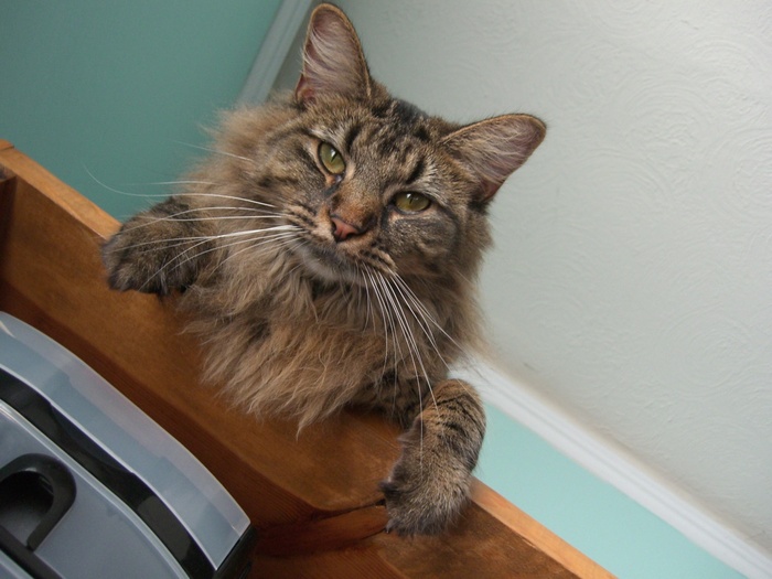
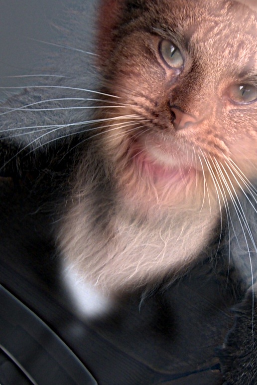
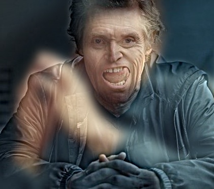
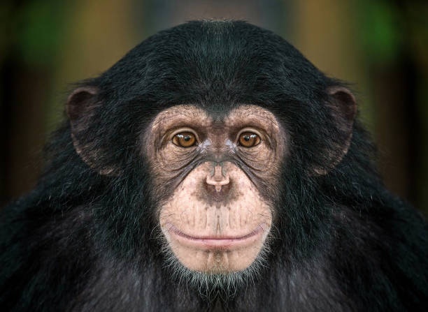
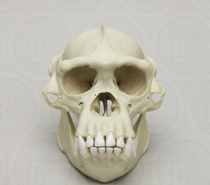
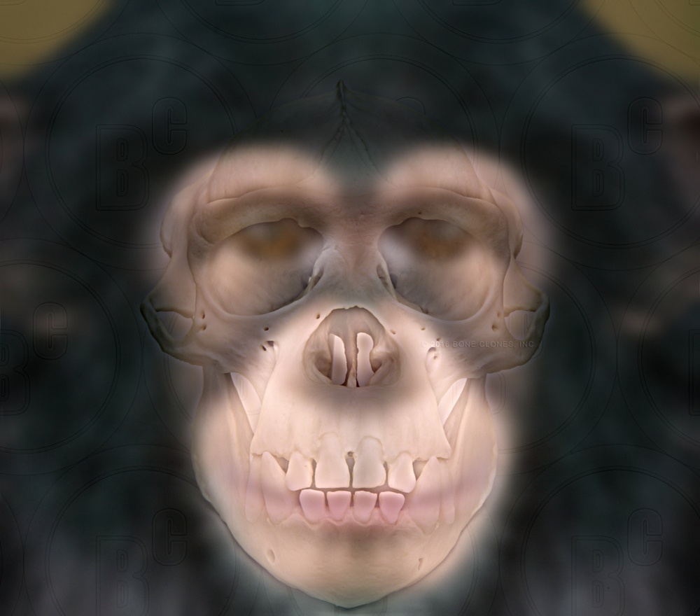
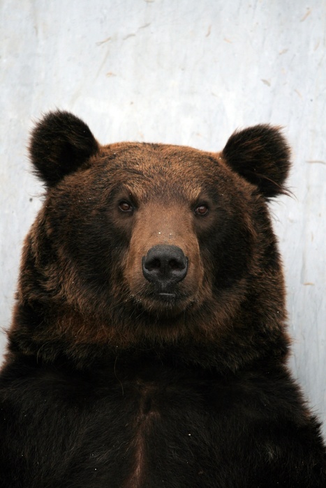
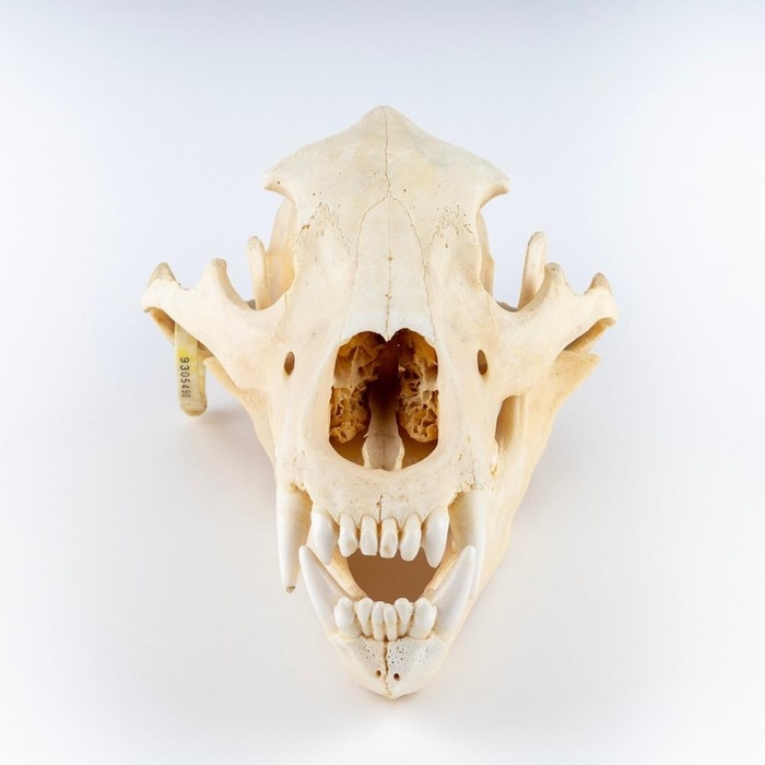
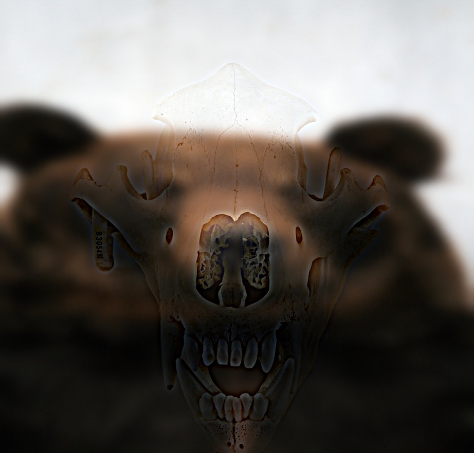
An x-ray variant for the animal skulls. For the chimp and the bear I deliberately gave up some of the clean switch. With the favorite's settings, the skull hides the animal completely up close. Moving the cutoffs to 16 / 28 c/i lets the animal's eyes, nose and lips survive in the low band. Scaling the high band by 0.8 (the per-band gain the paper mentions as an optional third parameter) tones the bone edges down. The result reads like an x-ray up close, with skull and face visible together, while from far away only the animal remains.
Part 2.2 Bells & Whistles: Where Should the Color Go?
I built every hybrid four ways: grayscale, color in the low-frequency image only, color in the high-frequency image only, and color in both. I also measured how much color each band carries, as the average spread between the R, G and B values at each pixel:
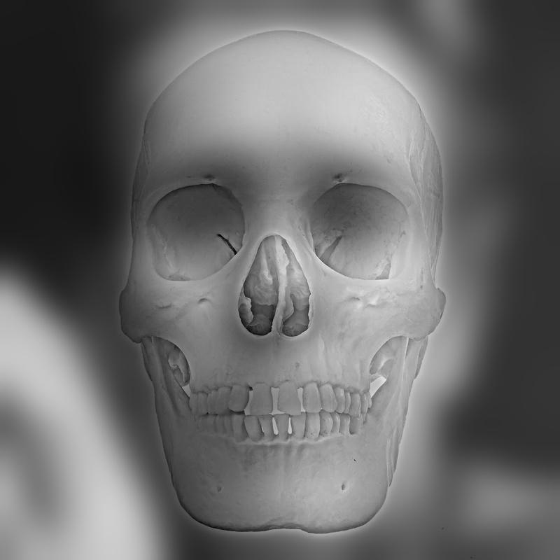
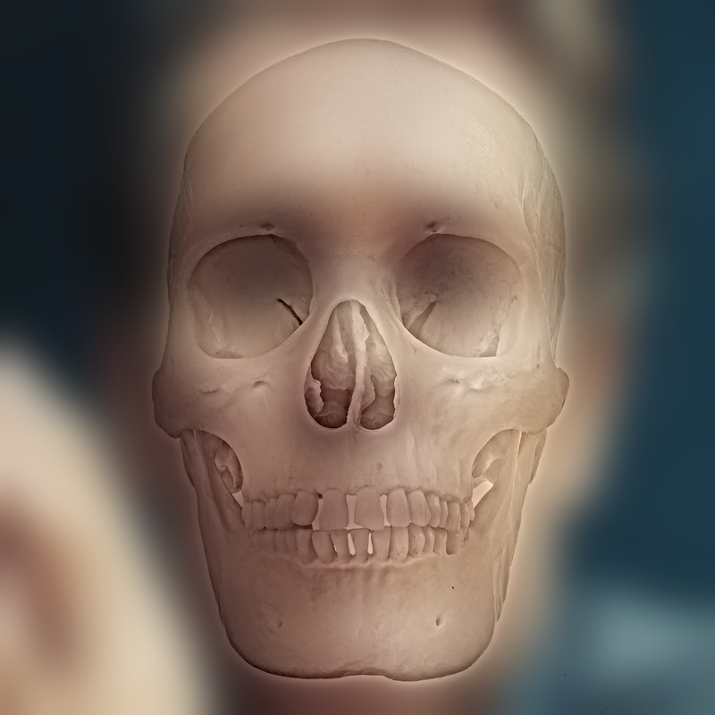
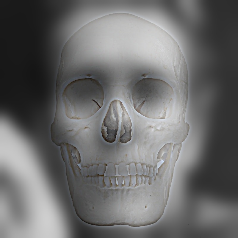
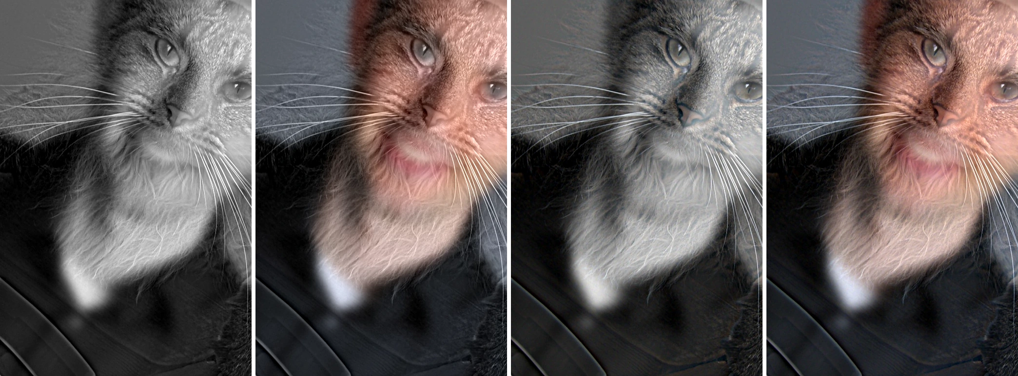
Color works best in the low-frequency image, and adding it to the high-frequency image contributes almost nothing. The reason is visible in the numbers: across all 6 hybrids, the high-pass band carries 5× to 21× less color than the low-pass band. Most of an object's color is its average, which is a low frequency, so the high-pass removes it along with the brightness. What is left of the high band is mostly how bright or dark each edge is, not what color it is. That also helps the illusion: the far image gets vivid color, which it needs since it has no sharp detail left, while the close-up image is carried by edges alone. The paper's bicycle example puts color in the high frequencies, but that works because the bicycle is a thin, saturated object whose color lives almost entirely in its fine structure. Skulls, fur and faces don't have that property.
Part 2.3: Gaussian and Laplacian Stacks
A pyramid halves the resolution at each level, so each level holds half the frequency range of the one above it. A stack keeps every level at full resolution. To make a stack behave like a pyramid, the total blur has to double from one level to the next, so I set
and build each level from the previous one by blurring with \(\sqrt{\sigma_k^2 - \sigma_{k-1}^2}\). That works because blurring twice, with σa and then σb, equals a single blur with \(\sqrt{\sigma_a^2 + \sigma_b^2}\). If I applied the same σ at every level instead, the total blur would only grow like \(\sqrt{k}\), and the coarse levels would never get coarse enough. With 7 levels and \(s_0 = 2\), the total σ per level is 0, 2, 4, 8, 16, 32, 64 px. Each Laplacian level is the difference of two neighboring Gaussian levels, and the last level keeps the remaining blurry image:
The sum telescopes, so the stack reconstructs the input exactly. The measured reconstruction error is 1.1 × 10⁻¹⁶. Everything is implemented from scratch, with no cv2.pyrDown or skimage pyramid functions. Long Gaussian kernels (the coarsest level of the 1600 px Manhattan blend uses σ = 256 px) are applied separably, one row pass and one column pass, via FFT convolution, which gives the same result to floating-point precision.
def gaussian_stack(im, levels, s0=1.0):
    sig = total_sigmas(levels, s0)
    stack = [im]
    for k in range(1, levels):
        inc = np.sqrt(sig[k] ** 2 - sig[k - 1] ** 2)
        stack.append(gaussian_blur(stack[-1], inc))
    return stack
def laplacian_stack(im, levels, s0=1.0):
g = gaussian_stack(im, levels, s0)
return [g[k] - g[k + 1] for k in range(levels - 1)] + [g[-1]], g




Recreating Szeliski Fig. 3.42
Rows one to three show Laplacian levels 0, 2, 4 (high, middle, and low frequencies). In each row, the left column is the apple band multiplied by the matching mask level, the middle is the orange band multiplied by one minus that mask, and the right is their sum. The last row adds up all levels. Each row shares one display scale.
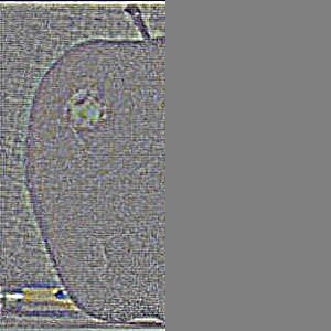
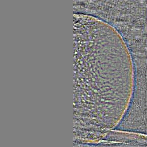
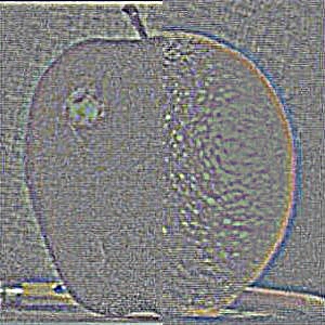
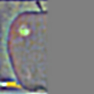
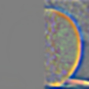
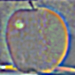
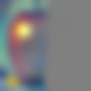
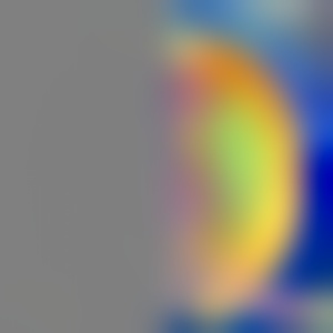
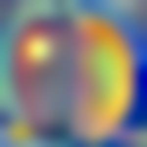
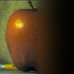
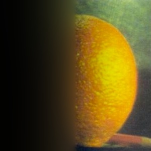
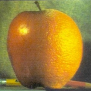
The key detail is how wide the seam is in each row. At L0 the mask is still nearly a hard step, so fine texture (the orange's pores, the apple's speckles) switches over within a couple of pixels. At L4 the mask has been blurred with σ = 2·2³ px, so the difference in overall color between the red apple and the yellow orange is spread across a wide band. Every frequency gets a transition width that matches its own scale.
Part 2.4: Multiresolution Blending (a.k.a. the Oraple!)
With stacks, the hard-seam algorithm on page 226 of Burt & Adelson does not work as-is. In a pyramid, the downsampling and upsampling blur the seam as a side effect, but a stack never resamples, so a hard seam would stay hard at every level. I therefore always use the masked version from page 230: build a Gaussian stack of the mask as well, and blend each Laplacian level with the matching mask level (mask = 1 selects image A):
def blend(im_a, im_b, mask, levels, s0=1.0, mask_s0=None, keep_bands=True):
    mask_s0 = s0 if mask_s0 is None else mask_s0
    sig, msig = total_sigmas(levels, s0), total_sigmas(levels, mask_s0)
    ga, gb, gm = im_a, im_b, mask
    out = np.zeros_like(im_a, dtype=np.float64)
    parts = {'a': [], 'b': [], 'out': [], 'mask': [],
             'sum_a': np.zeros_like(out), 'sum_b': np.zeros_like(out)}   # masked inputs, all levels
    for k in range(levels):
        if k < levels - 1:
            na = gaussian_blur(ga, np.sqrt(sig[k + 1] ** 2 - sig[k] ** 2))
            nb = gaussian_blur(gb, np.sqrt(sig[k + 1] ** 2 - sig[k] ** 2))
            nm = gaussian_blur(gm, np.sqrt(msig[k + 1] ** 2 - msig[k] ** 2))
            la, lb = ga - na, gb - nb
        else:
            la, lb = ga, gb
        m = expand_mask(gm, im_a)
        band_a, band_b = m * la, (1 - m) * lb
        out += band_a + band_b
        parts['sum_a'] += band_a
        parts['sum_b'] += band_b
        if keep_bands:
            parts['a'].append(band_a)
            parts['b'].append(band_b)
            parts['out'].append(band_a + band_b)
            parts['mask'].append(gm)
        if k < levels - 1:
            ga, gb, gm = na, nb, nm
    return np.clip(out, 0, 1), parts
The oraple, and why multiresolution
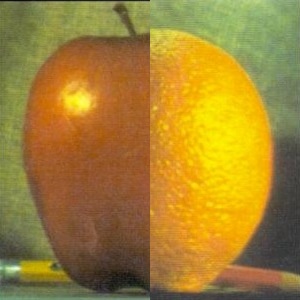
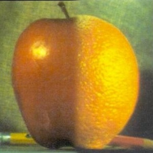
Here is the same vertical step mask applied three ways. A hard cut shows a visible seam. A single feathered alpha blend has to compromise on one transition width: too narrow and the color jump shows, too wide and the fine textures overlap into a double exposure. The multiresolution blend doesn't have to compromise, because each frequency band gets its own transition width.
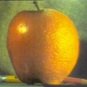
My blends
| Blend | Size | Mask | Mask area | Levels | Coarsest σ |
|---|---|---|---|---|---|
| Oraple | 300×300 | step (vertical) | 50% | 7 | 64 px |
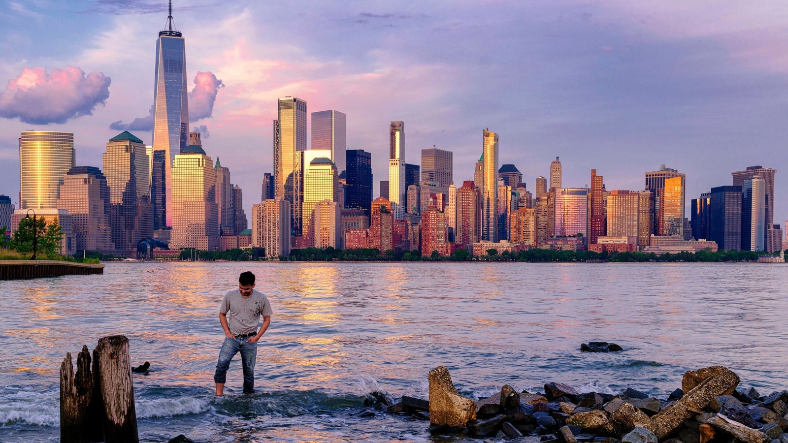
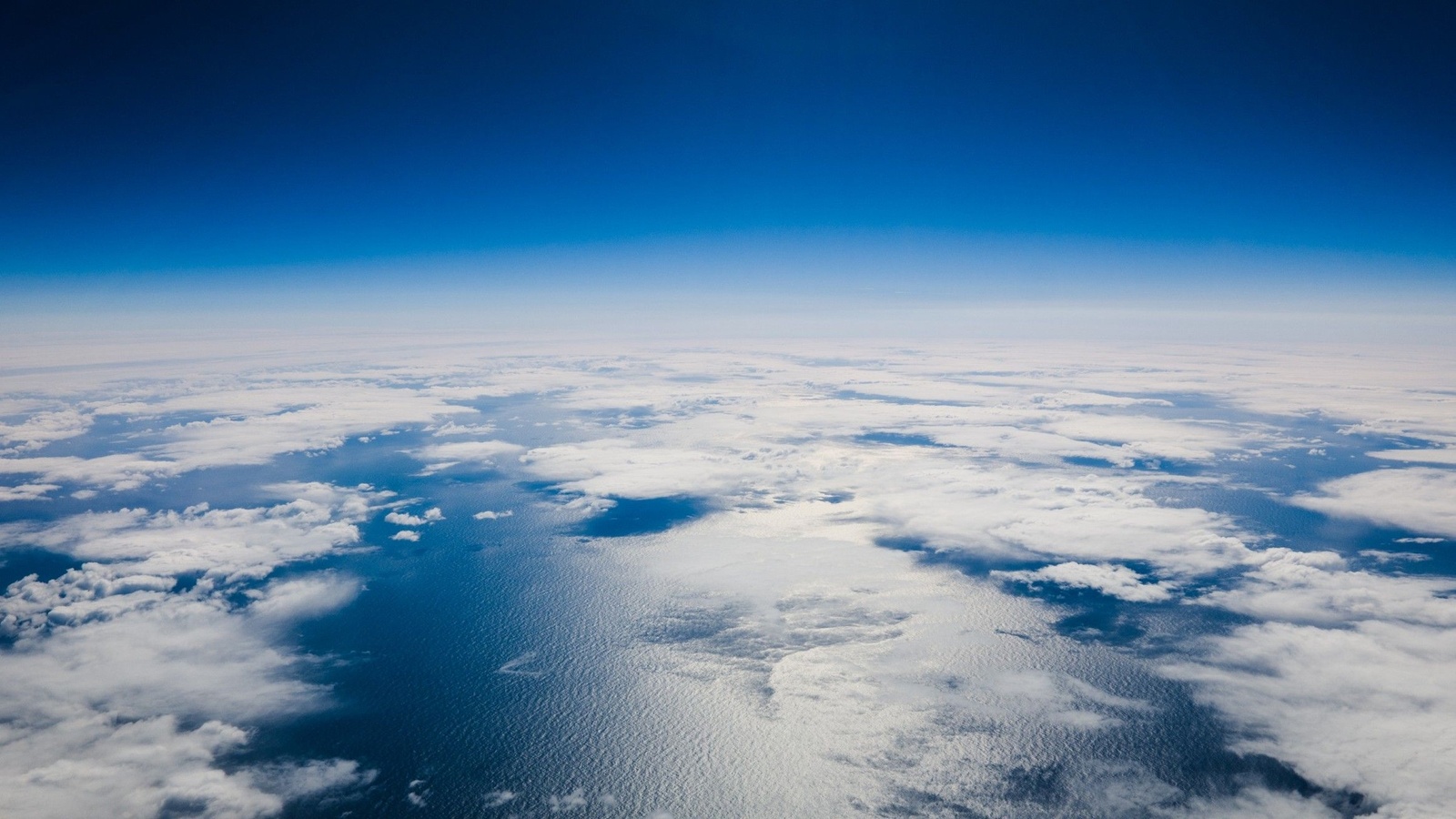
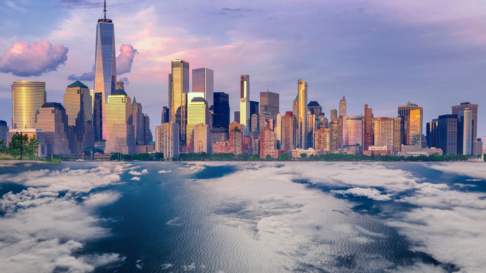
| Manhattan above the clouds | 1600×900 | step (horizontal) | 60% | 9 | 256 px |
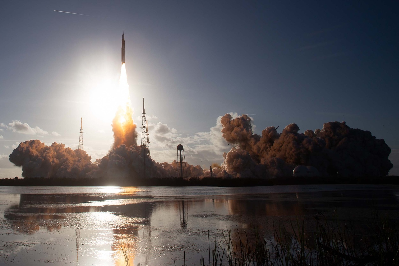
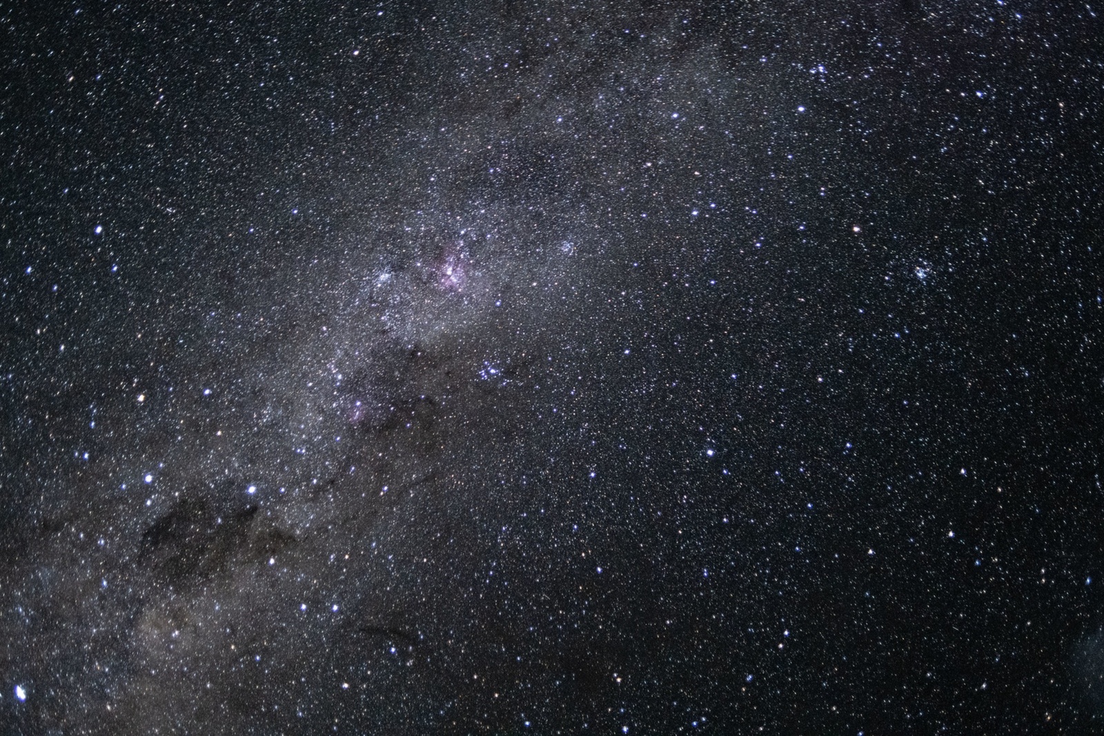
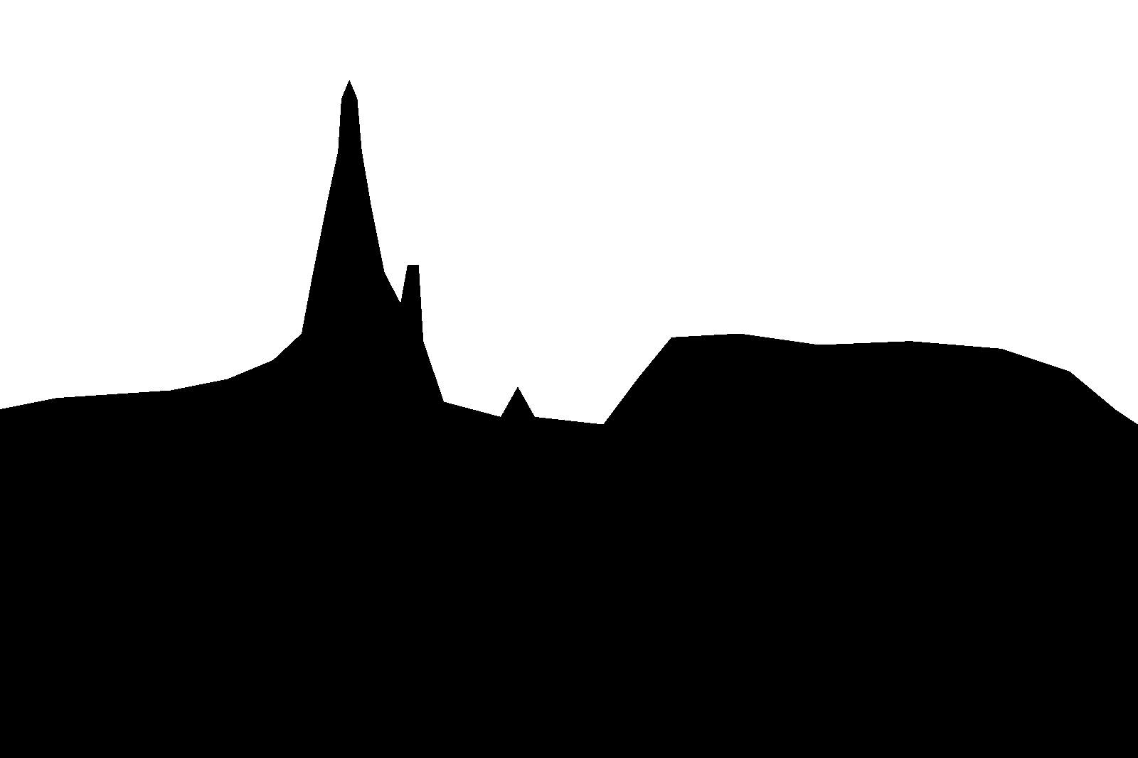
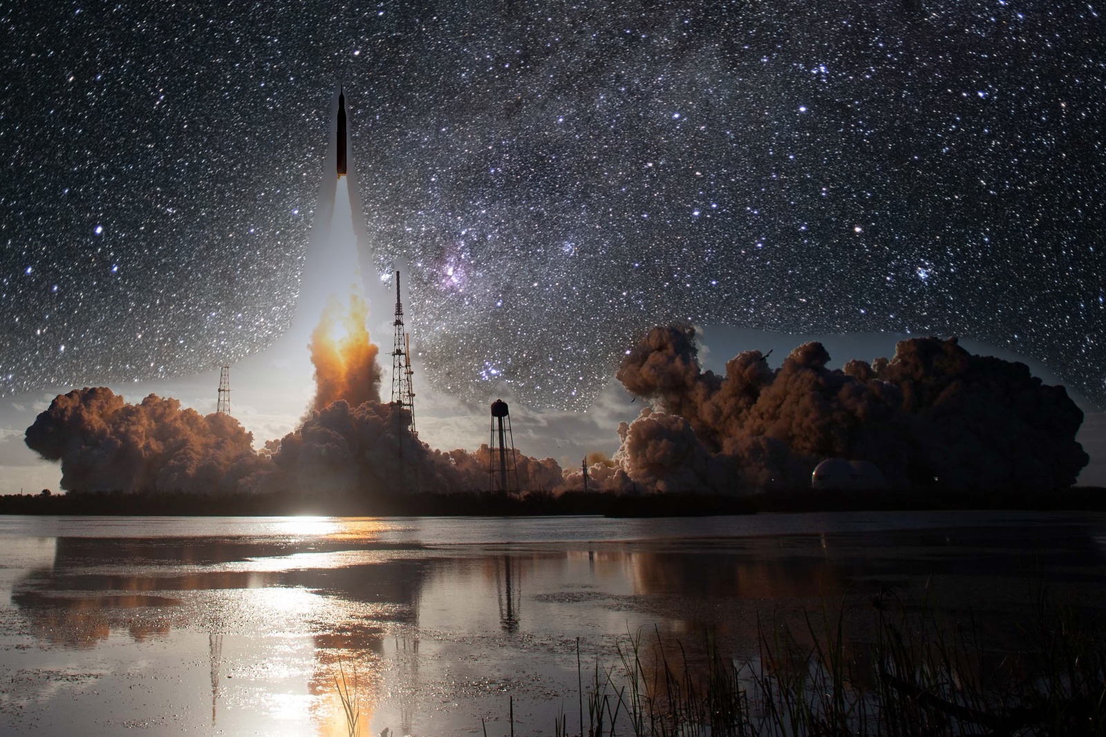
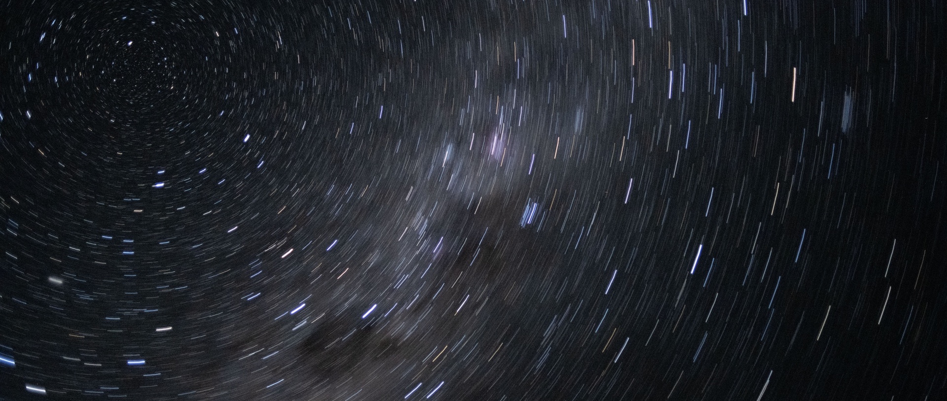
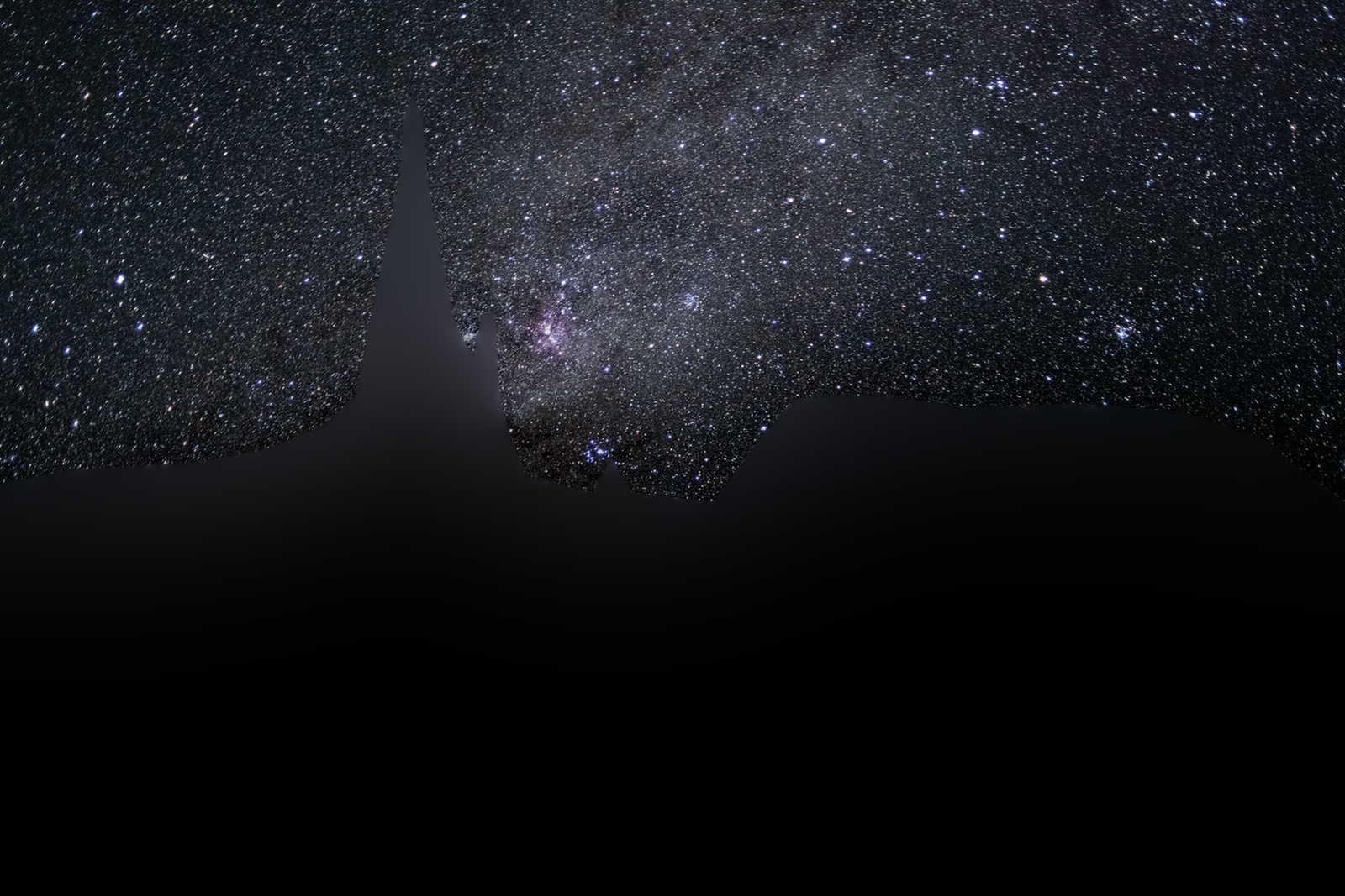
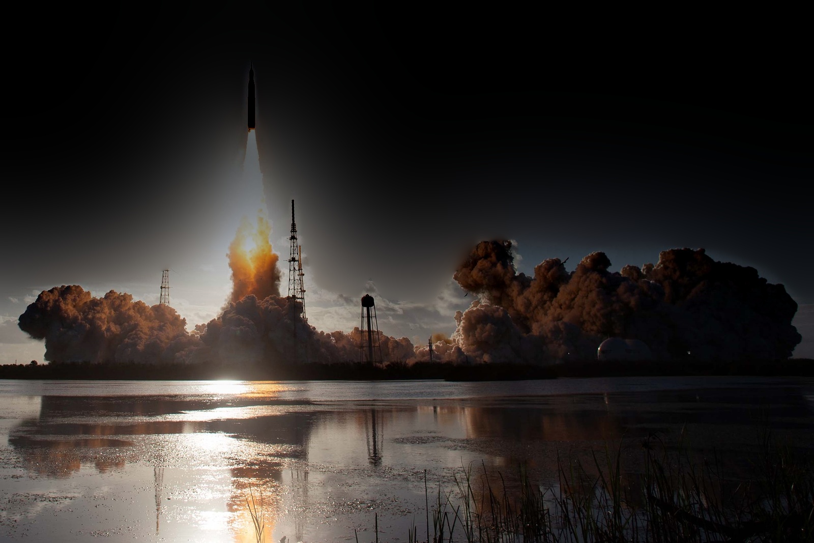
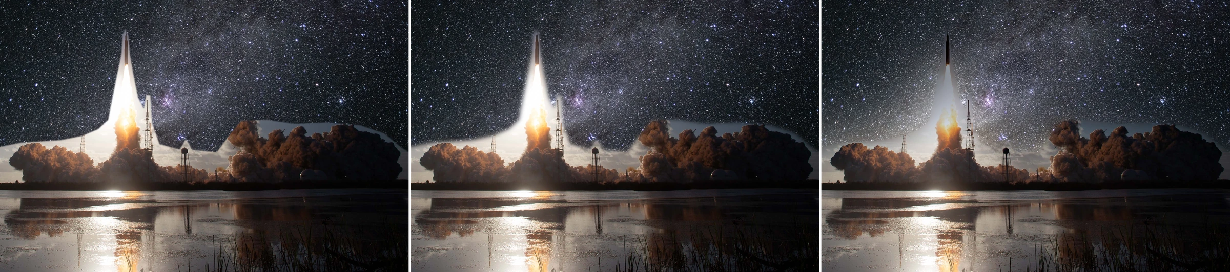
| Launch into the Milky Way | 1600×1067 | hand-traced polygon | 47% | 8 | 128 px |
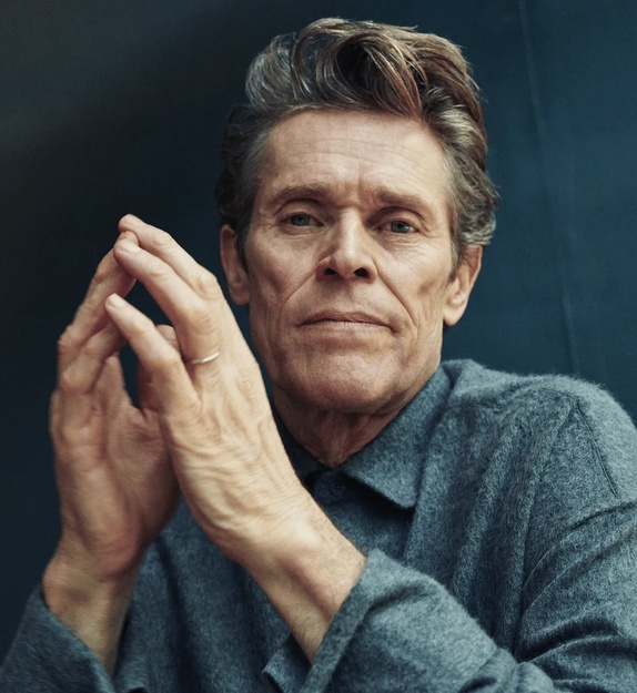
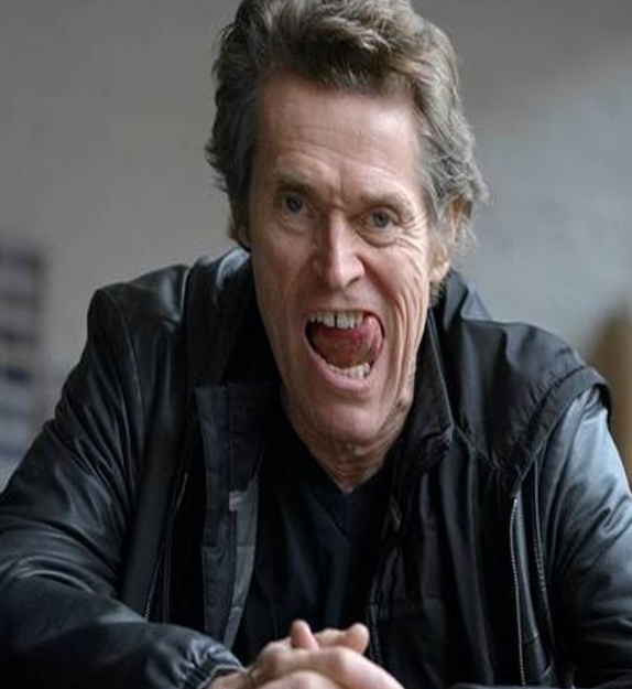
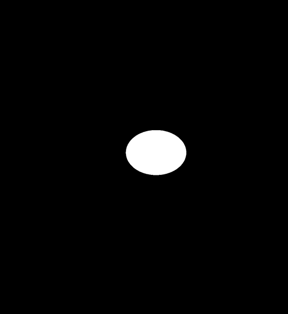
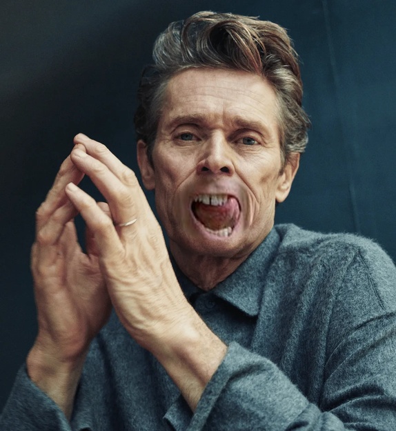
| Mouth transplant | 574×625 | ellipse, warped with its photo | 2% | 5 | 12 px |
| Beard transplant | 763×763 | hand-traced polygon, warped with its photo | 7% | 4 | 6 px |
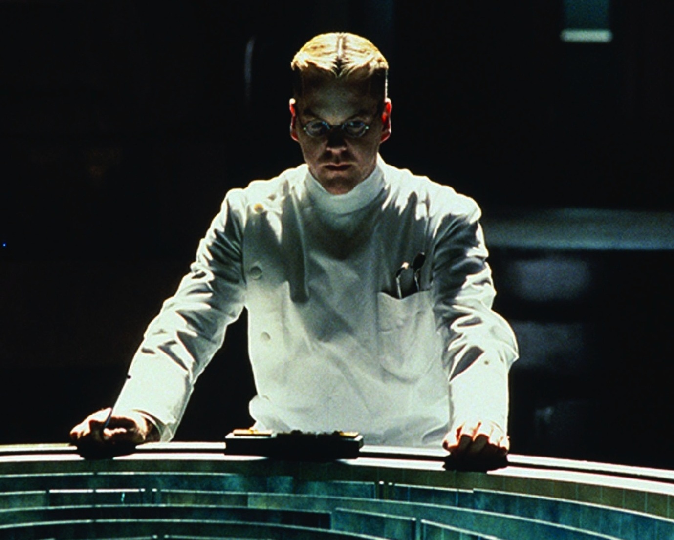
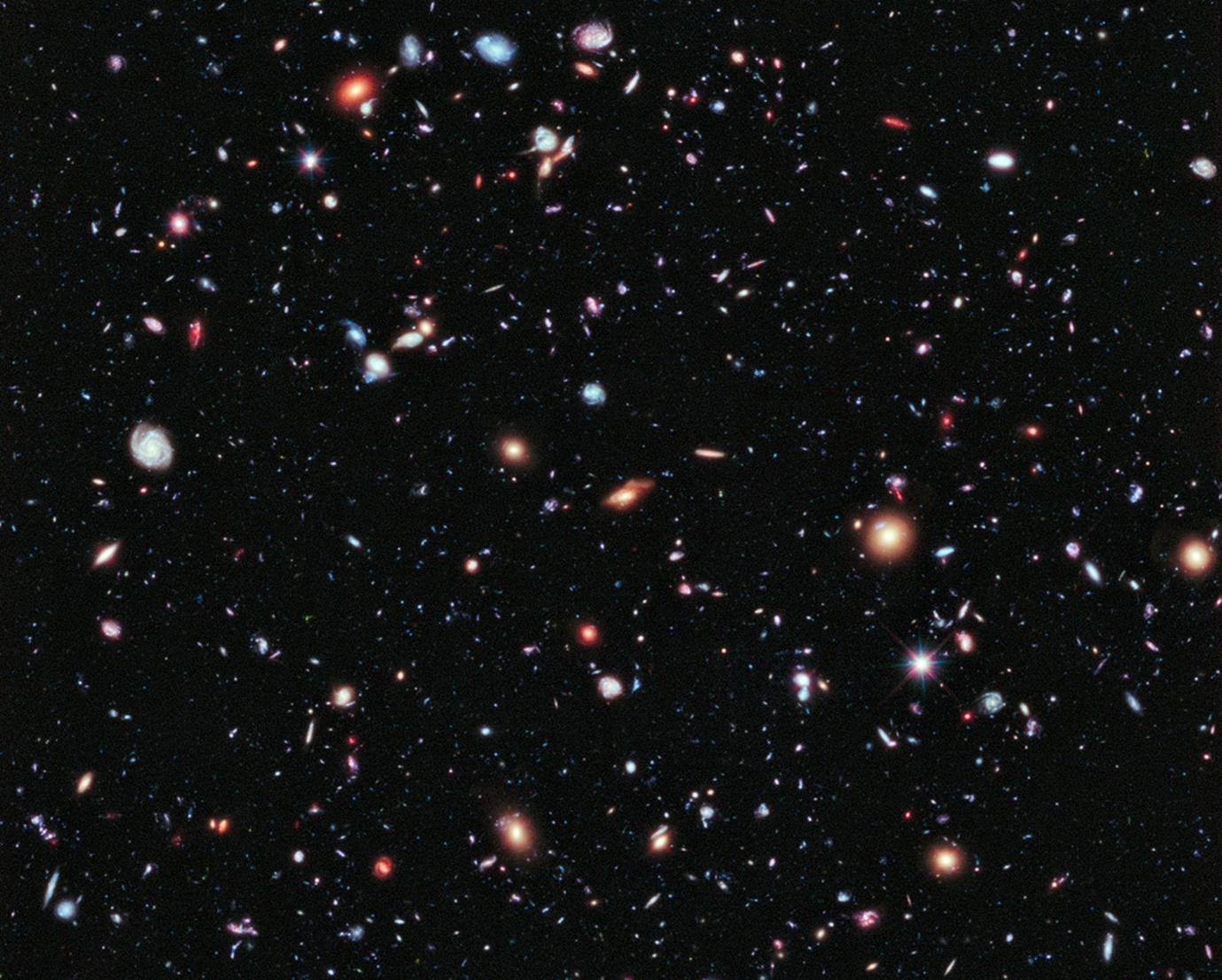
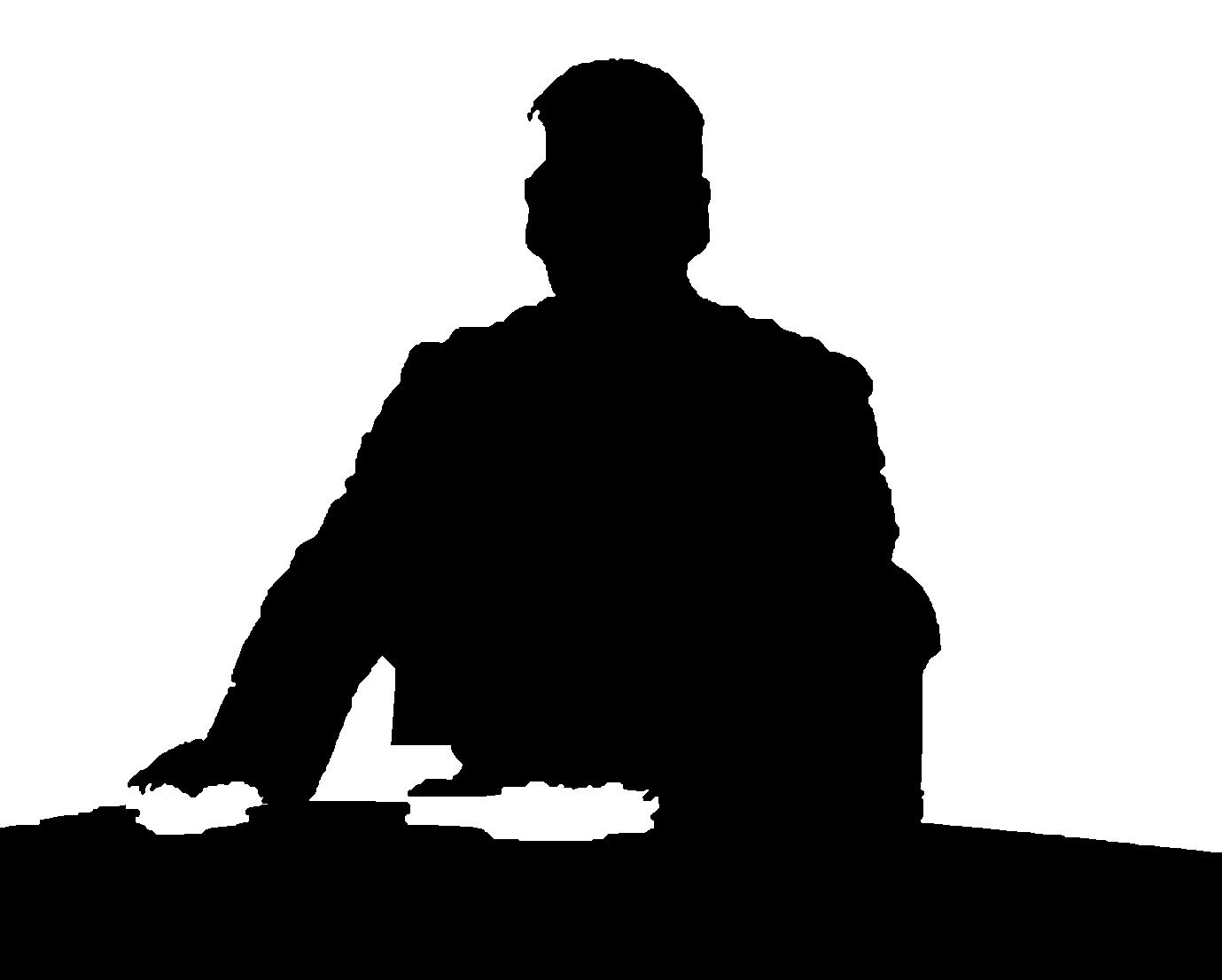
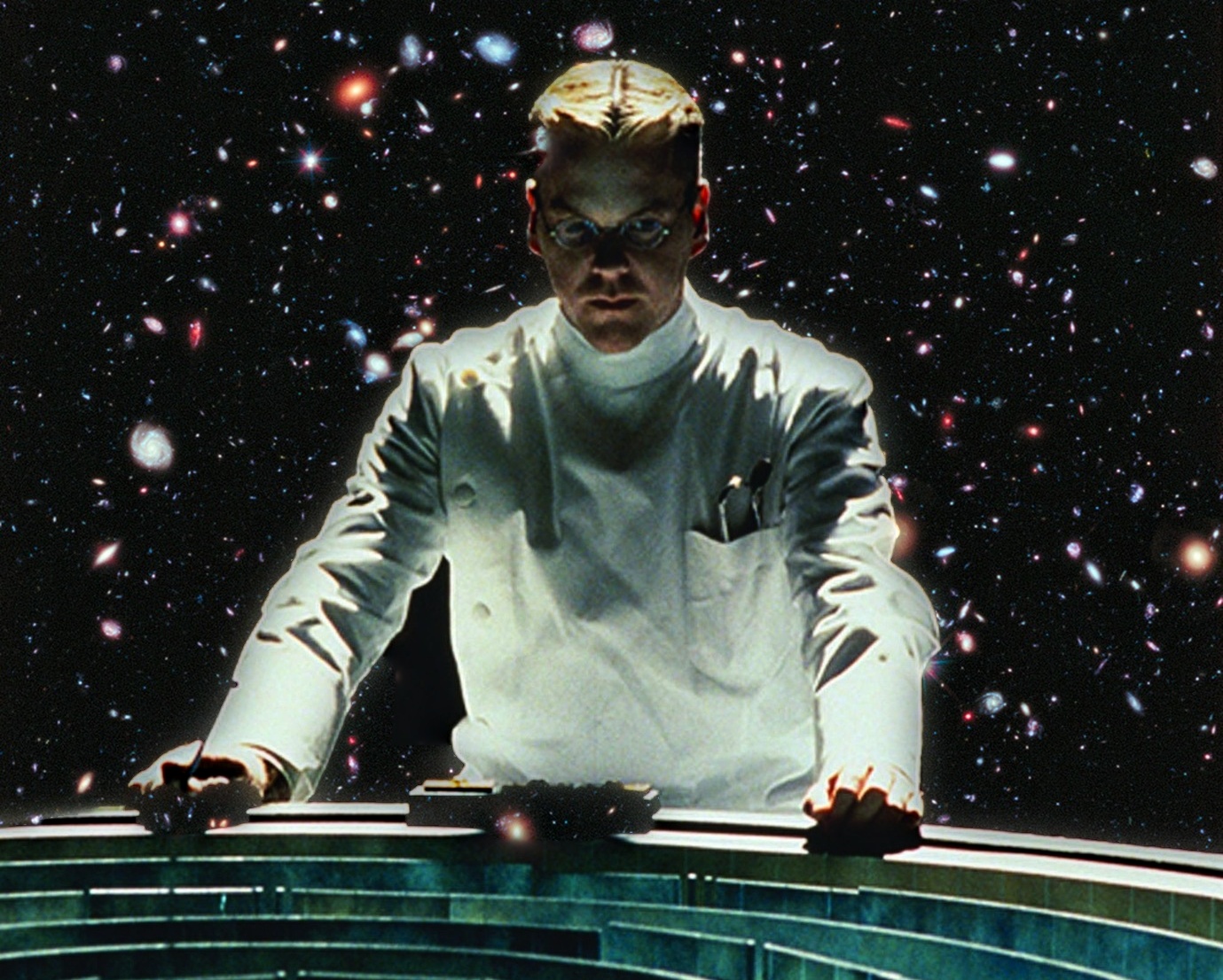
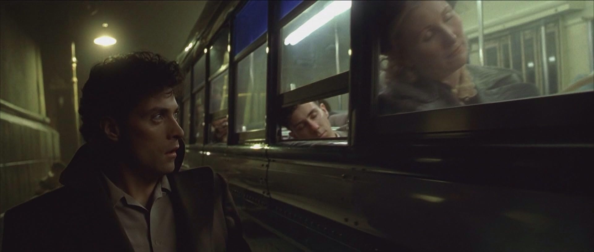
| Dark City: the doctor in deep space | 1379×1106 | rough outline + GrabCut | 57% | 6 | 24 px |
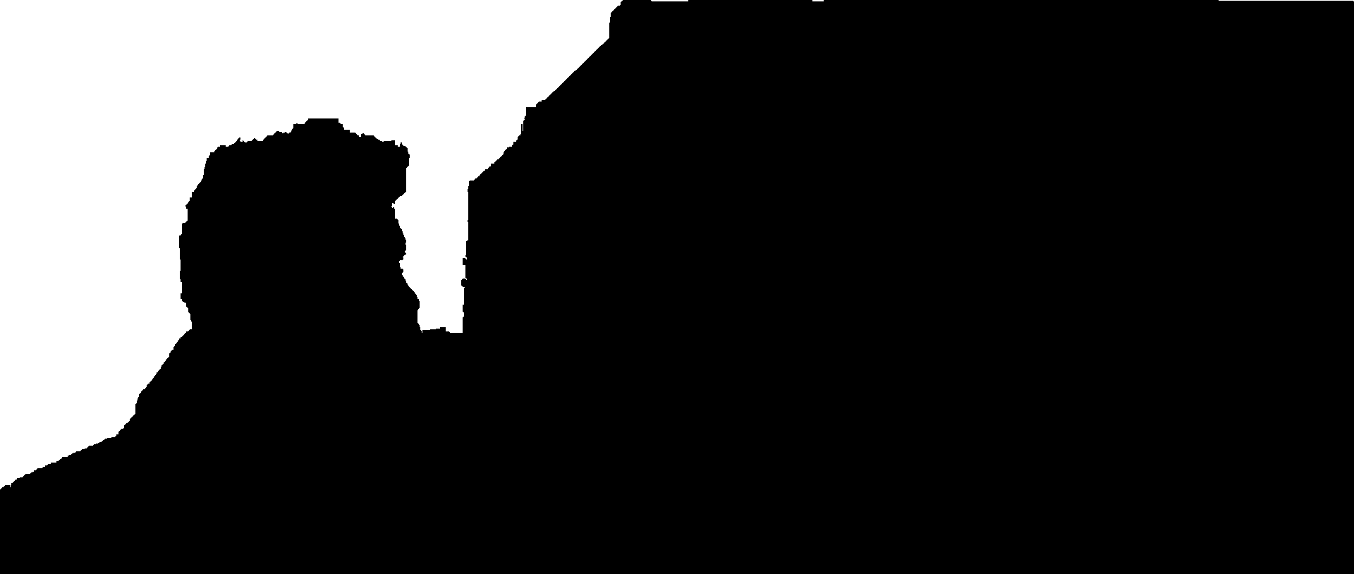
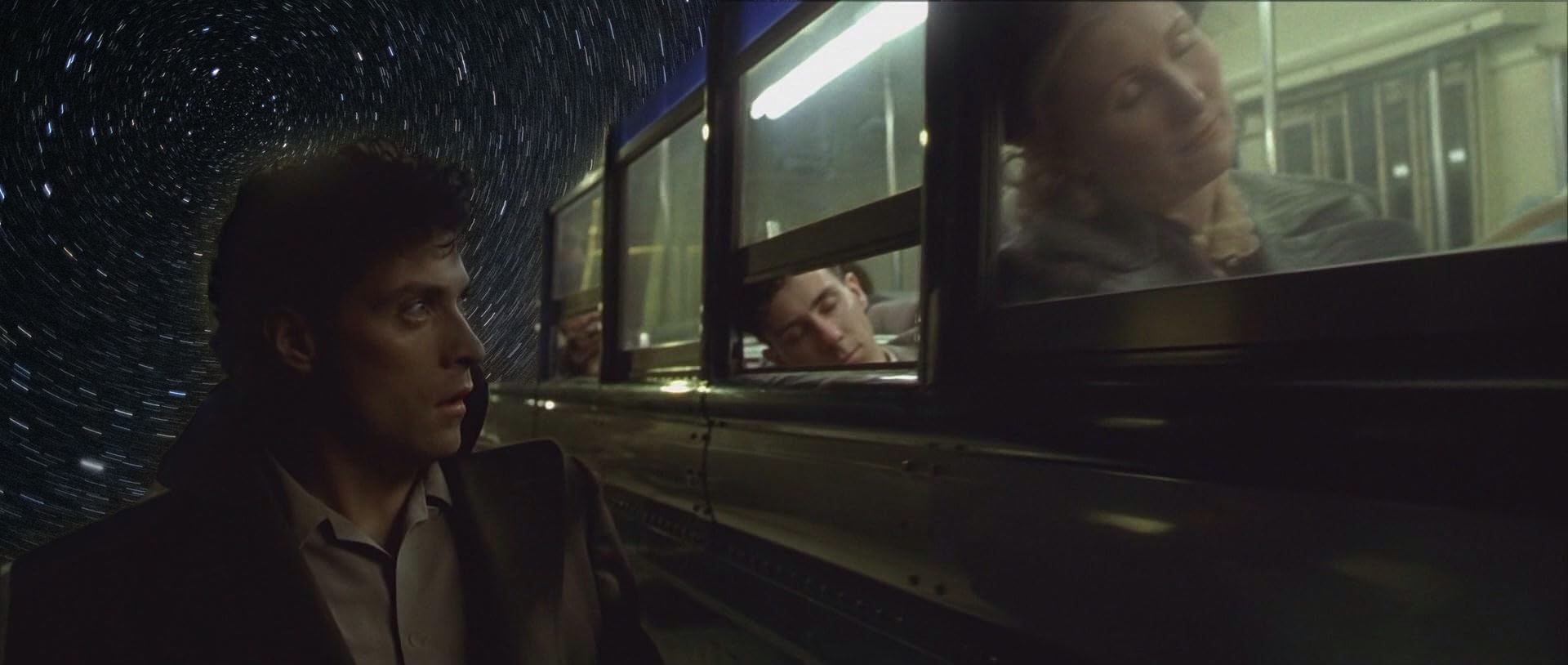
| Dark City: the night train under star trails | 1920×814 | rough outline + GrabCut | 19% | 6 | 24 px |
Most of my masks needed more than a straight line:
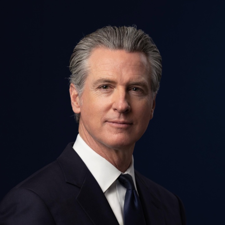
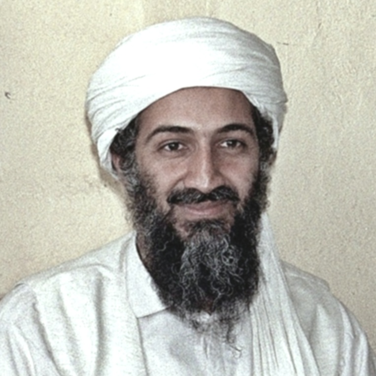
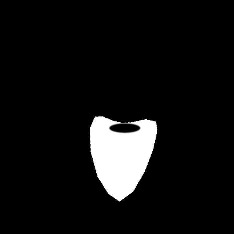
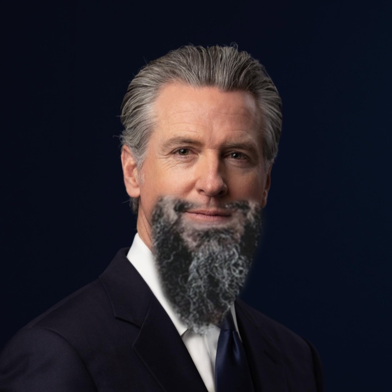
- Face swaps. The mask has to stay on the face through alignment, so it is drawn on the source photo and warped along with it, carried as a fourth image channel through the same transform. The mouth swap uses the hybrids' three-point affine alignment (eyes plus mouth). For the beard, a rotation-and-scale-only (similarity) fit to the same three points works better: with three points the affine fit matches them exactly and spends its extra freedom on shear, slanting the face, while the similarity fit needs only a 4.6° turn. The beard mask also has a hole cut around Newsom's own lips, so only the mustache and beard come from bin Laden. I capped the upsampling of the lower-resolution face at 1.5×, blurred the old bin Laden scan with σ = 1 to remove film grain, and corrected its colors before blending (below).
- Dark City. These masks have to follow a person's outline. I traced a rough polygon around the subject, and GrabCut (OpenCV's graph-cut segmentation) refined it to the real silhouette, including the hair, the sleeves, and the gap between the arm and the coat. Only then does the mask go into the stacks.
Straight seam · Manhattan above the clouds

Irregular mask · Launch into the Milky Way (favorite)
Irregular mask · Mouth transplant
Irregular mask · Beard transplant
Irregular mask · Dark City: the doctor in deep space
Irregular mask · Dark City: the night train under star trails
The beard also shows the main limit of the method. Blending smooths the transition between two images at every scale, but it does not make their colors agree, because inside the mask the result simply is image A. The old scan had a strong cool cast and colored grain in the hair, so I corrected it before blending. I measured the average Lab color of matching skin patches on both faces (forehead and nose), shifted bin Laden's whole photo by the difference, and kept 35% of its chroma so the hair reads as neutral salt-and-pepper. Shifting only the averages, and not the contrast, keeps the beard dark. When I also matched the contrast, it washed out to a gray haze.
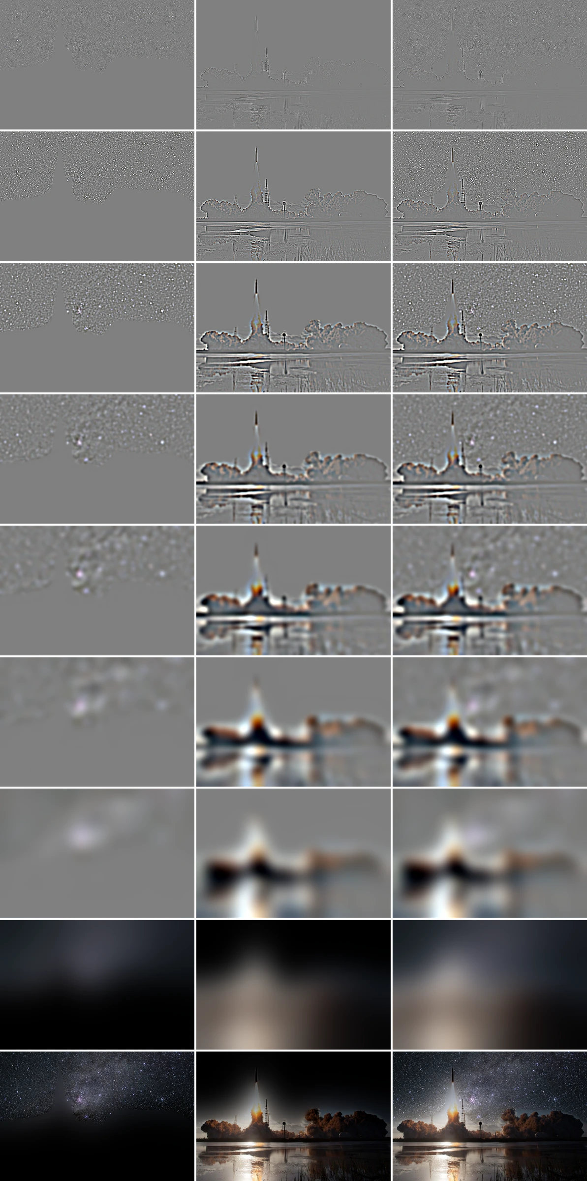
Laplacian stack of my favorite blend
This is the same breakdown as Burt & Adelson's Figure 10, for the launch. Each row is one level from fine (top) to coarse, with the masked stars, the masked launch photo, and their sum. The last two rows are the remaining blurry level and the sum of all levels.
Part 2.4 Bells & Whistles: Color and Stack Depth
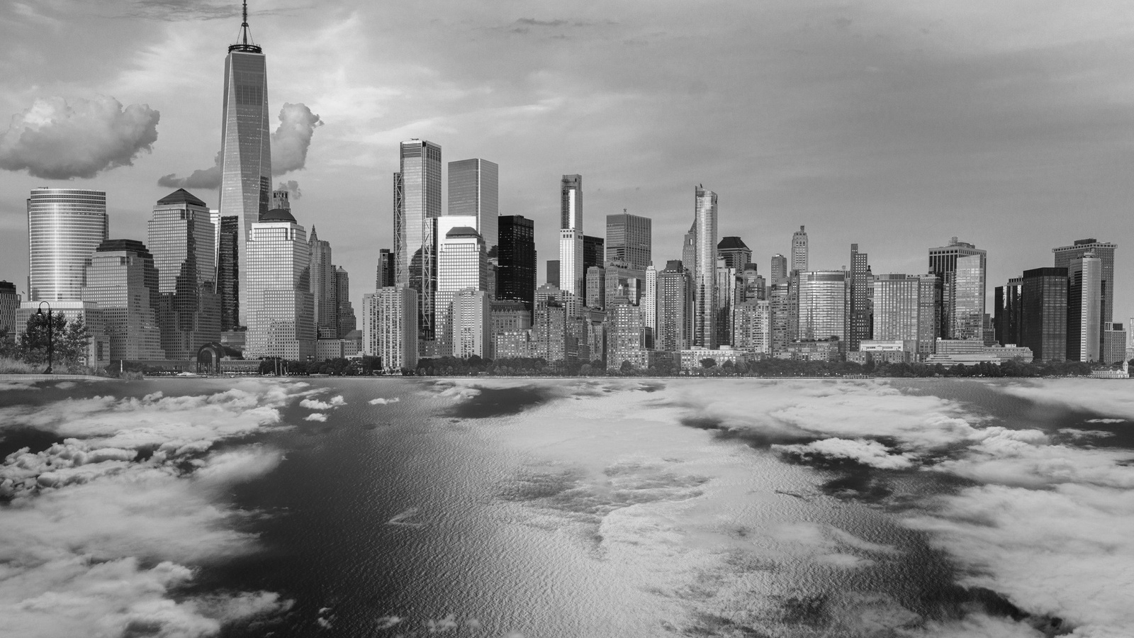
Color. All blends above are done in color, by running the stacks on each RGB channel separately. Blending the grayscale versions instead removes the main thing that makes Manhattan above the clouds believable: the purple sunset sky and the blue cloud layer shift their colors gradually through the coarse levels. In gray, the scene is readable but flat, and the atmosphere is gone.
Stack depth. Adding more levels extends the widest transition, since the coarsest mask level's σ doubles with each level. To check this with numbers, I measured the average gradient in a band around the mask edge, where a visible seam shows up as extra gradient:
| Blend | Shallow (levels) | Medium (levels) | Full depth (levels) | Change |
|---|---|---|---|---|
| Oraple | 0.0421 (2) | 0.0374 (4) | 0.0351 (7) | −17% |
| Manhattan above the clouds | 0.1080 (2) | 0.1018 (4) | 0.0978 (9) | −9% |
| Launch into the Milky Way | 0.1021 (2) | 0.0899 (4) | 0.0774 (8) | −24% |
| Mouth transplant | 0.0641 (2) | 0.0597 (4) | 0.0590 (5) | −8% |
| Beard transplant | 0.0586 (2) | 0.0530 (4) | −10% | |
| Dark City: the doctor in deep space | 0.1223 (2) | 0.1036 (4) | 0.0943 (6) | −23% |
| Dark City: the night train under star trails | 0.0476 (2) | 0.0447 (4) | 0.0443 (6) | −7% |
Going from two levels to the full depth lowers the seam gradient by 7% to 24% in every blend. The gain is largest for the launch into the milky way (24%) and the doctor in deep space (23%), where large bright and dark regions meet along the seam. It is smallest for the the night train under star trails (7%) and mouth transplant (8%), where the mask follows a small or detailed outline and there is little low-frequency difference to smooth. That is also why I did not use maximum depth everywhere: once the coarsest level is wider than the region being pasted, the pasted image's surroundings start to leak out. That was the white glow I first got around the beard, and it is why the face swaps and the Dark City cut-outs use fewer levels.
What I Learned
The most important thing I learned is that every part of this project is the same idea: deciding what happens to each frequency band. Edge detection differentiates the image but has to suppress the highest band, or noise wins. Sharpening boosts the upper band, and it can only boost what the blur left behind. A hybrid image hands the low band to one picture and the high band to another, and it only works when the two bands are kept apart. Blending gives each band its own seam width. Once I started thinking in terms of "which frequencies, and how wide," the parameters stopped being magic numbers. Alignment turned out to matter just as much: a third point and an affine warp did more for the skulls and the face swaps than any filter setting. The cutoff gap, the threshold after smoothing, and the stack depth all had reasons I could explain and measure.
The implementation lesson was just as concrete: with Python loops, the question is not how many loops you have but how much work each iteration does. The same two-loop count was either 6.8× faster than the four-loop version or 3.0× slower, depending on whether the remaining loop ran over pixels or over kernel taps.